Q1. Some of your data in Column C is displaying as hashtags (#) because the column is too narrow. How can you widen Column C just enough to show all the data?
- Right-click column C, select Format Cells, and then select Best-Fit.
- Right-click column C and select Best-Fit.
- Double-click column C.
- Double-click the vertical boundary between columns C and D.
- ISNUMBER and ISTEXT
- ISNUMBER and ISALPHA
- ISVALUE AND ISNUMBER
- ISVALUE and ISTEXT
Q3. If you drag the fill handle (lower-right corner) of cell A2 downward into cells A3, A4, and A5, what contents will appear in those cells?

- Jan, Jan, Jan
- Feb, Mar, blank cell
- Feb, Mar, Apr
- FEB, MAB, APR
- the death of chivalry
- The death of Chivalry
- THE DEATH OF CHIVALRY
- The Death Of Chivalry
Q5. In the worksheet below, you want to use Data > Subtotal to show a subtotal value per sport. What must you do BEFORE applying the Subtotal function?

- Sort by the data in Column E.
- Format the data in Column D.
- Sort by the data in Column D.
- Format the data in Column E.
Q6. When editing a cell, what do you press to cycle between relative, mixed, and absolute cell references?
- Alt+F4 (Windows) or Option+F4 (Mac)
- Alt+Shift+4 (Windows) or Option+Shift+4 (Mac)
- Ctrl+Shift+4 (Windows) or Command+Shift+4 (Mac)
- the F4 (Windows) or Command+T (Mac)
Q7. You need to add a line chart showing a sales trends over the last 12 months and you have only a little space to work with. How can you convey the required information within a single cell?
- Add an image of the chart to a comment.
- Add a hyperlink to another worksheet that displays a chart when clicked.
- Add an image of the chart to the worksheet.
- Add a sparkline, a graphic that summarizes data visually within a single worksheet cell.
- Right-click anywhere and select Help.
- Press F1 or click the Help tab in the ribbon.
- Press F10.
- all of these answers.
- ##,###,,
- ###.0,,
- 999.9,,
- ###,###.0,
- three inputs
- four inputs
- two inputs
- one input
Q11. In the image below, which option(s) can you select so that the appropriate field headers appear in cells A4 and B3 instead of the terms Row Labels and Column Labels, respectively?

- Show in Tabular Form
- Show in Compact Form
- Show in Compact For or Show in Outline Form
- Show in Tabular Form or Show in Outline Form
Q12. A cell contains the value 7.877 and you want it to display as 7.9. How can you accomplish this?
- Use the ROUND() function.
- Click the Decrease Decimal button twice.
- In the cells group on the Home tab, click Format > Format Cells. Then click the Alignment tab and select Right Indent.
- Click the Decrease Decimal button once.
- =A3+A4+A5+A6
- =SUM(A3:A6)
- =SUM(A3,A6)
- =SUM(A3,A4,A5,A6)
Q14. Which custom format will make the cells in column A appear like the corresponding cells in column B?
- MMM-YYYY
- MMMM-YYYY
- MMMM&"-"&YYYY
- M-YYYY
Q15. Which function returns a reference to a cell (or cell range) that is a specified distance from a base cell?
- OFFSET
- VLOOKUP
- INDEX
- MATCH
Q16. You're working with columns whose width and font-size should not be changed. Yet the columns are too narrow to display all the text in each cell. What tool should you use to solve the problem?
- Sparklines
- Wrap Text
- Fill Handle
- Centered Alignment
- pie chart
- line chart
- XY scatter chart
- bar chart

- The AutoSum formulas refer to the column to the left of their cells.
- The AutoSum formulas exclude the bottom row of data.
- The AutoSum formulas include the year at the top of each column in the calculation.
The formula bar clearly shows it's the dates (top row) included, along with the total (bottom) row. Thus, the bottom row of data is not excluded. - The AutoSum formulas include their own cells, creating a circular reference.
Q19. The text filter in column A is designed to display only those rows where column A entry has a particular attribute. What is this attribute?

- The second character in the cell is 9.
- The number 9 appears one or more times within the cell.
- The cell is comprised of 9 characters.
- The number 9 appears once and only once within the cell.
Q20. To ensure shapes and other objects are an equal left-to-right distance apart, select the shapes, click Page Layout > Align, and then click ____.
- Align Middle
- Distribute Horizontally
- Distribute Vertically
- Align Center
Q21. An organization chart, which shows the hierarchy within a company or organization, is available as ___ that is included with Excel.
- a 3D model
- SmartArt
- a Treemap chart
- a drawing object
Q22. You want to be able to restrict values allowed in a cell and need to create a drop-down list of values from which users can choose. Which feature should you use?
- Protect Worksheet
- Conditional Formatting
- Allow Users to Edit Ranges
- Data Validation
Q23. To round up a value to the nearest increment of your choice, such as the next five cents, what function should you use?
- ROUNDUP
- MAX
- ROUND
- CEILING
- =MAX(H2:H30)
- =MAXIMUM(H2:H30)
- =LARGE(H2:H30,29)
- =UPPER(H2:H30,1)
Q25. Which chart type can display two different data series as a different series type within the same chart?
- XY chart
- clustered column
- bubble chart
- combo chart

- Hides or shows the formula bar.
- Selects all.
- Hides or shows the ribbon.
- Selects objects.
- =MySheet!A1
- =MySheet_A1
- =MySheet&A1
- =MySheet@A1
Q28. In the worksheet below, you want to copy the formatting of cell A1 into cells B1:D1. Which approach (see arrows) accomplishes this the most efficiently?

- B
- C
- A
- D
- =COUNT(B4:E4&G4:I4)
- =COUNT(B4:E4,G4:I4)
- =COUNT(B4:E4 G4:I4)
- =COUNT(B4:I4)
- In the Format group, select Trendline from the Insert Shapes list.
- Click outside the plot area and select Add Trendline
- Click inside the plot and select Forecast.
- Right-click a data series and select Add Trendline.
- Goal Seek
- Power Pivot
- Data Analysis
- Solver
- Protect Workbook
- Watch Window
- Data Validation
- Filter
Q33. You want to apply subtotals per sport in the data below. What should you do before applying subtotals?
- Format the data in column E.
- Format the data in column D.
- Sort the data in column D.
- Sort the data in column E.
Q34. When you sort a list of numerical value into ascending or descending order, the value in the middle of the list is the ___.
- mode
- modulus
- average
- median
- Cell style
- Fill color
- Pattern style
- Font color
- :
- =
- (
- -
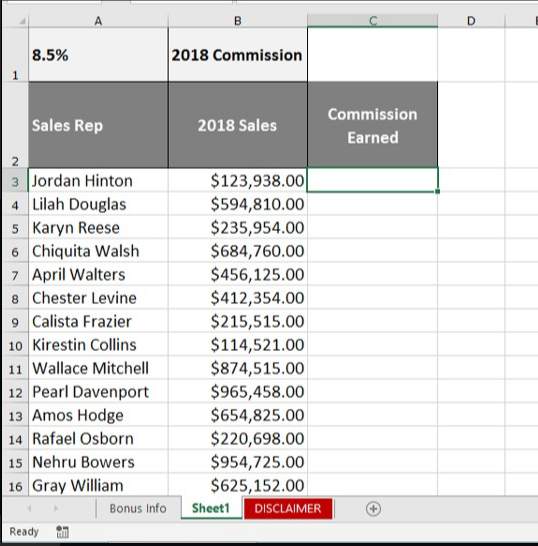
Q37. You need to determine the commission earned by each Sales Rep, based on the Sales amounts in B3:B50 and the Commission rate specified in cell A1. You want to enter a formula in C3 and copy it down to C50. Which formula should you use?
| A | B | C | |
|---|---|---|---|
| 1 | 8.5% | 2018 Commission | |
| 2 | Sales Rep | 2018 Sales | Commission Earned |
| 3 | Jordan Hinton | $123,938.00 | |
| 4 | Lilah Douglas | $5594,810.00 | |
| 5 | Karyn Reese | $235,954.00 | |
| 6 | Chiquita Walsh | $684,760.00 |
- =$A1*B3
- =$A$1*B3
- =A1*$B3
- =A1*B3
Q38. If you start a date series by dragging down the fill handle of a single cell that contains the date 12/1/19, what will you get?
- a series of consecutive days following the initial date
- a series of days exactly one month apart
- a series of days identical to the initial date
- a series of days exactly one year apart
Q39. To discover how many cells in a range contain values that meet a single criterion, use the ___function.
- COUNT
- SUMIFS
- COUNTA
- COUNTIF
Q40. Your worksheet has the value 27 in cell B3. What value is returned by the function =MOD (B3,6)?
- 4
- 1
- 5
- 3
Q41. For an IF function to check whether cell B3 contains a value between 15 and 20 inclusively, what condition should you use?
- OR(B3=>15,B3<=20)
- AND (B3>=15,B3<=20)
- OR(B3>15,B3<20)
- AND(B3>15, B3<20)
- Fill color
- Font Color
- Pattern Style
- Cell Style
Q43. The charts below are based on the data in cells A3:G5. The chart on the right was created by copying the one on the left. Which ribbon button was clicked to change the layout of the chart on the right?

- Move Chart
- Switch Row/Column
- Quick Layout
- Change Chart Type
Q44. Cell A20 displays an orange background when its value is 5. Changing the value to 6 changes the background color to green. What type of formatting is applied to cell A20?
- Value Formatting
- Cell Style Formatting
- Conditional Formatting
- Tabular format
- It adds data from cell D18 of Sheet1 and cell D18 of Sheet4
- It adds data from cell A1 of Sheet1 and cell D18 of sheet4
- It adds all data in the range A1:D18 in Sheet1, Sheet2, Sheet3 and Sheet4
- It adds data from all D18 cells in Sheet1, Sheet2, Sheet3 and Sheet4
Q46. What is the term for an expression that is entered into a worksheet cell and begins with an equal sign?
- function
- argument
- formula
- contents
- In a worksheet cell, array formulas have a small blue triangle in the cell's upper-right corner.
- A heavy border appears around the range that is occupied by the array formula.
- In the formula bar, an array formula appears surrounded by curly brackets.
- When a cell that contains an array formula is selected, range finders appear on the worksheet around the formula's precedent cells.
Q48. In a worksheet, column A contains employee last names, column B contains their middle initials (if any), and column C contains their first names. Which tool can combine the last names, initials, and first names in column D without using a worksheet formula?
- Concatenation
- Columns to Text
- Flash Fill
- AutoFill
- ='Budget Variances'!A10
- ='Budget Variances!A10'
- ="BudgetVariances!A10"
- ="BudgetVariances"!A10
- =FIND(A1,1,5)
- =SEARCH(A1,5)
- =LEFT(A1,5)
- =A1-RIGHT(A1,LEN(A1)-5)
- =ISALPHA(A1)
- =ISCHAR(A1)
- =ISSTRING(A1)
- =ISTEXT(A1)
- =UPPER(H2:30,1)
- =MAXIMUM(H2:H30)
- =MAX(H2:H30)
- =LARGE(H2:H30,29)
Q53. You select cell A1, hover the pointer over the cell border to reveal the move icon, then drag the cell to a new location. Which ribbon commands achieve the same result?
- Cut and Fill
- Cut and Paste
- Copy and Transpose
- Copy and Paste
Q54. You want to add a column to the PivotTable below that shows a 5% bonus for each sales rep. That data does not exists in the original data table. How can you do this without adding more data to the table?
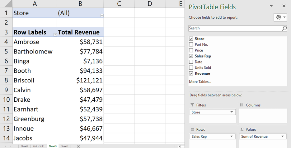
- Add a new PivotTable field.
- Add a calculated item
- Add a new Summarize Value By field.
- Add a calculated field.
Q55. You need to determine the commission earned by each Sales rep, based on the Sales amount in B3:B50 and the Commission rate specified in cell A1. You want to enter a formula in C3 and copy it down to C50. Which formula should you use?
- =A1*$B3
- =A1*B3
- =$A$1*B3
- =$A1*B3
Q56. The NOW() function returns the current date and time as 43740.665218. Which part of this value indicates the time?
- 6652
- 43740.665218
- 43740
- 665218
Q57. Cell A2 contains the value 8 and cell B2 contains the value 9. What happens when cells A2 and B2 are merged and then unmerged?
- Both values are lost.
- Cell A2 contains the value 8 and cell B2 is empty.
- Cell A2 contains the value 8 and cell B2 contains the value 9.
- Cell A2 contains the value 17 and cell B2 is empty.
- column D
- columns D through H
- column H
- column F
- cell values only
- cell values and formats
- cell values and formulas
- cell value, formats, and formulas
Q60. Which function, when entered into cell G7, allows you to determine the sum total of annual sles for market regions 18 and greater?

-
=SUMIF(G2:G6,">17",F2:F6) -
=SUM(G2:G6,">=18,F2:F6) -
=SUMIF(F2:F6,">=18",G2:G6) -
=SUM(F2:F6,"18+",G2:G6)
Q61. Which function, when entered into cell F2 and then dragged to cell F6, returns the performance rating text (e.g., "Good", "Poor") for each representative?

-
=RIGHT(E2,LEN(E2)-27) -
=LEN(E2,MID(E2)-27) -
=LEFT(E2,LEN(E2)-27) -
=RIGHT(E2,MID(E2)-27)
=SUMIFS(Colors[Inventory],Colors[Colors],"Orange")
- the Inventory worksheet in the Colors workbook
- the Inventory column in the Colors table
- the Colors worksheet in the Inventory workbook
- the named range Colors[Inventory], which does not use Format as Table Feature
Q63. Which VLOOKUP function, when entered into cell L2 and then dragged to cell L5, returns the average number of calls for the representative IDs listed in column J?

-
=VLOOKUP(A2,J2:L5,1,FALSE) -
=VLOOKUP(J2,A$2:C$7,1,FALSE) -
=VLOOKUP(J2,A$2:C$7,3,FALSE) -
=VLOOKUP(J2,A2:C7,3,FALSE)
because we are interested in the value of the 3rd column of the table
-
=SUBTOTAL(C1:Y15) -
=SUM(15L:15Z) -
=SUM(C15:Y15) -
=SUM(C11:C35)
the sum of columns C to Y for the same row 15

- 4
- 5
- 3
- 2

- Select
Paste Special > Values. - Select
Paste Special > Transpose. - Use the
TRANSPOSEfunction - Click
Switch Rows & Columns
because it needs to be transposed without creating a reference
-
=RIGHT(A1)-LEFT(A1)+1 -
=LEN(A1) -
=EXACT(A1) -
=CHARS(A1)
Q68. Which formula, when entered into cell D2 and then dragged to cell D6, calculates the average total number of minutes spent on phone calls for each representative?

-
=B$2*C$2 -
=$C$2/$B$2 -
=C2/B2 -
=B2*C2
Q69. The PivotTable below has one row field and two column fields. How can you pivot this table to show the column fields as subtotals of each value in the row field?

- On the PivotTable itself, drag each
Averagefield into the row fields area. - Right-click a cel in the PivotTable and select
PivotTable Options > Classic PivotTable layout. - In the
PivotTable Fieldspane, dragSum Valuesfrom theColumnssection to a location below the field in theRowssection. - In the
PivotTable Fieldspane, drag each field from theSum Valuessection to theRowssection.

- grouping
- filtering
- hiding
- cut and paste
Q71. Monthly revenues of 2019 are entered in B2:M2, as shown below, To get year-to-date running total revenues, what formula should you enter in B3 and autofill through M3?

-
=SUMIF($B$2:$M$2,"COLUMN($B$2:$M$2)<=COLUMN())") -
=SUM($B2:B2) -
=SUM(OFFSET($A1,0,0,1,COLUMN())) -
=B2+B3
we are calculating the running total here
- 4
- 1
- 5
- 3
- rows:event, donor / values: Sum of amount
- columns: event / row:donor / values: Sum of amount
- rows:donor, event / values: Sum of amount
- filter: event / row:donor / values: Sum of amount
Q74. In the worksheet shown below, cell C6 contains the formula=VLOOKUP(A6,$F$2:$G$10,2,FALSE). What is the most likely reason that #N/A is returned in cell C6 instead of mallory's ID (2H54)
- The absolute/relative cell references in the formula are wrong
- Cell A6 is not actualy text its a formula that need to be copied and pasted as a value
- Column C in the lookup range is not sorted properly
- A trailing space probably exist in cell A6 or F7
Q75. What is the difference between pressing the delete key and using the clear command in the Home tab's Editing group?
- deletes removes the entire column or row. Clear removes the content from the column or row
- deletes removes formulas, values and hyperlinks. clear removes formulas, values, hyperlinks, formats, comments and notes
- Delete removes the cell itself, shifting cells either up or to the left. Clear removes content and properties but does not muves cells
- Delete removes formulas and values. clear removes formulas, values, hyperlinks, formats, comments and notes
- cell
- selection
- element
- scalar