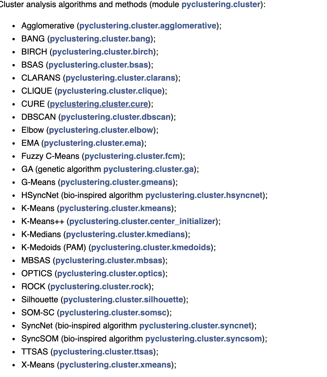
- Vidhya on clustering and methods
- KNN intuition 2, thorough explanation 3 - classify a new sample by looking at the majority vote of its K-nearest neighbours. k=1 special case. Even amount of classes needs an odd K that is not a multiple of the amount of classes in order to break ties.
- Determinging the number of clusters, a comparison of several methods, elbow, silhouette etc
- A good visual example of kmeans / gmm
- Kmeans with DTW, probably fixed length vectors, using tslearn
- Kmeans for variable length, notebook
TOOLS
- Any of the “precomputed” algorithms in sklearn, just remember to do 1-distanceMatrix. I.e., using dbscan/hdbscan/optics, you need a dissimilarity matrix.
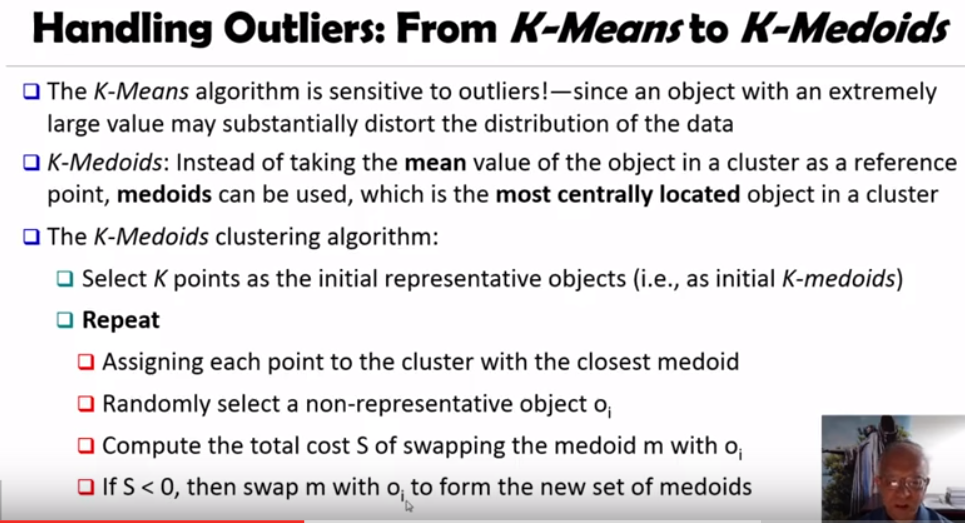
- Sensitive to outliers, can skew results (because we rely on the mean)
- basically k-means with a most center object rather than a center virtual point that was based on mean distance from all points, we keep choosing medoids samples based on minimised SSE
- k-medoid is a classical partitioning technique of clustering that clusters the data set of n objects into k clusters known a priori.
- It is more robust to noise and outliers as compared to k-means because it minimizes a sum of pairwise dissimilarities instead of a sum of squared Euclidean distances.
- A medoid can be defined as the object of a cluster whose average dissimilarity to all the objects in the cluster is minimal. i.e. it is a most centrally located point in the cluster.
- Does Not scale to many samples, its O(K*n-K)^2
- Randomized resampling can assure efficiency and quality.
- "Python implementations of the k-modes and k-prototypes clustering algorithms, for clustering categorical data" - git
- a guide to clustering mixed types, i.e., numerics, categoricals
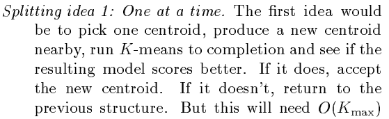
X-means(paper): \
- Theory behind bic calculation with a formula.
- Code: Calculate bic in k-means
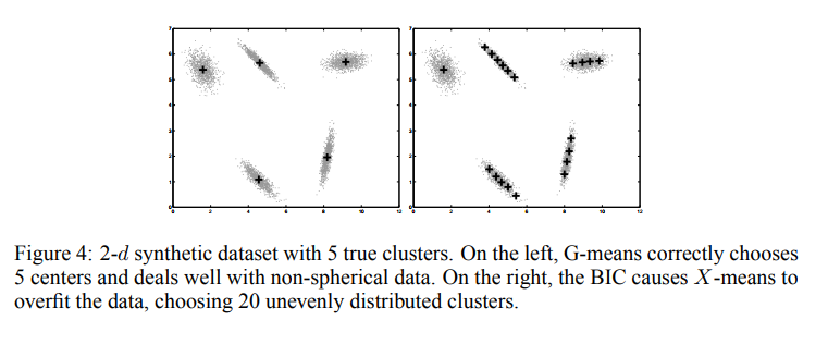
G-means Improves on X-means in the paper: The G-means algorithm starts with a small number of k-means centers, and grows the number of centers. Each iteration of the algorithm splits into two those centers whose data appear not to come from a Gaussian distribution using the Anderson Darling test. Between each round of splitting, we run k-means on the entire dataset and all the centers to refine the current solution. We can initialize with just k = 1, or we can choose some larger value of k if we have some prior knowledge about the range of k. G-means repeatedly makes decisions based on a statistical test for the data assigned to each enter. If the data currently assigned to a k-means center appear to be Gaussian, then we want to represent that data with only one center.
?- What is GMM in short its knn with mean/variance centroids, a sample can be in several centroids with a certain probability.\
Let us briefly talk about a probabilistic generalisation of k-means: the Gaussian Mixture Model(GMM).
In k-means, you carry out the following procedure:
- specify k centroids, initialising their coordinates randomly
- calculate the distance of each data point to each centroid
- assign each data point to its nearest centroid
- update the coordinates of the centroid to the mean of all points assigned to it
- iterate until convergence.
In a GMM, you carry out the following procedure:
- specify k multivariate Gaussians (termed components), initialising their mean and variance randomly
- calculate the probability of each data point being produced by each component (sometimes termed the responsibility each component takes for the data point)
- assign each data point to the component it belongs to with the highest probability
- update the mean and variance of the component to the mean and variance of all data points assigned to it
- iterate until convergence
You may notice the similarity between these two procedures. In fact, k-means is a GMM with fixed-variance components. Under a GMM, the probabilities (I think) you're looking for are the responsibilities each component takes for each data point.\
- Gmm code on sklearn using ellipsoids
- How to select the K using bic
- Density estimation for gmm - nice graph
- A comparison of kmeans++ vs kernel kmeans
- Kernel Kmeans is part of TSLearn
- Elbow method,
- elbow and mean silhouette,
- elbow on medium using mean distance per cluster from the center
- Kneed a library to find the knee in a curve
- Nearpy, knn in scale! On github
- finding the optimal K
- Benchmark of nearest neighbours libraries
- billion scale aprox nearest neighbour search
- How to use effectively
- a DBSCAN visualization - very good!
- DBSCAN for GPS.
- A practical guide to dbscan - pretty good
- Custom DBSCAN “predict”
- Haversine distances for dbscan
- Optimized dbscans:
- muDBSCAN, paper - A fast, exact, and scalable algorithm for DBSCAN clustering. This repository contains the implementation for the distributed spatial clustering algorithm proposed in the paper μDBSCAN: An Exact Scalable DBSCAN Algorithm for Big Data Exploiting Spatial Locality
- Dbscan multiplex - A fast and memory-efficient implementation of DBSCAN (Density-Based Spatial Clustering of Applications with Noise).
- Fast dbscan - A lightweight, fast dbscan implementation for use on peptide strings. It uses pure C for the distance calculations and clustering. This code is then wrapped in python.
- Faster dbscan paper
(what is?) HDBSCAN is a clustering algorithm developed by Campello, Moulavi, and Sander. It extends DBSCAN by converting it into a hierarchical clustering algorithm, and then using a technique to extract a flat clustering based in the stability of clusters.
- Github code
- (great) Documentation with examples, for clustering, outlier detection, comparison, benchmarking and analysis!
- (jupytr example) - take a look and see how to use it, usage examples are also in the docs and github
What are the algorithm’s steps:
- Transform the space according to the density/sparsity.
- Build the minimum spanning tree of the distance weighted graph.
- Construct a cluster hierarchy of connected components.
- Condense the cluster hierarchy based on minimum cluster size.
- Extract the stable clusters from the condensed tree.
(What is?) Ordering points to identify the clustering structure (OPTICS) is an algorithm for finding density-based[1] clusters in spatial data
- Its basic idea is similar to DBSCAN,[3]
- it addresses one of DBSCAN's major weaknesses: the problem of detecting meaningful clusters in data of varying density.
- (How?) the points of the database are (linearly) ordered such that points which are spatially closest become neighbors in the ordering.
- a special distance is stored for each point that represents the density that needs to be accepted for a cluster in order to have both points belong to the same cluster. (This is represented as a dendrogram.)
An SVM-based clustering algorithm is introduced that clusters data with no a priori knowledge of input classes.
- The algorithm initializes by first running a binary SVM classifier against a data set with each vector in the set randomly labelled, this is repeated until an initial convergence occurs.
- Once this initialization step is complete, the SVM confidence parameters for classification on each of the training instances can be accessed.
- The lowest confidence data (e.g., the worst of the mislabelled data) then has its' labels switched to the other class label.
- The SVM is then re-run on the data set (with partly re-labelled data) and is guaranteed to converge in this situation since it converged previously, and now it has fewer data points to carry with mislabelling penalties.
- This approach appears to limit exposure to the local minima traps that can occur with other approaches. Thus, the algorithm then improves on its weakly convergent result by SVM re-training after each re-labeling on the worst of the misclassified vectors – i.e., those feature vectors with confidence factor values beyond some threshold.
- The repetition of the above process improves the accuracy, here a measure of separability, until there are no misclassifications. Variations on this type of clustering approach are shown.
Constrained K-means algorithm, git, paper, is a semi-supervised algorithm.\
Clustering is traditionally viewed as an unsupervised method for data analysis. However, in some cases information about the problem domain is available in addition to the data instances themselves. In this paper, we demonstrate how the popular k-means clustering algorithm can be profitably modified to make use of this information. In experiments with artificial constraints on six data sets, we observe improvements in clustering accuracy. We also apply this method to the real-world problem of automatically detecting road lanes from GPS data and observe dramatic increases in performance.
\
In the context of partitioning algorithms, instance level constraints are a useful way to express a priori knowledge about which instances should or should not be grouped together. Consequently, we consider two types of pairwise constraints:
• Must-link constraints specify that two instances have to be in the same cluster.
• Cannot-link constraints specify that two instances must not be placed in the same cluster.