🚀 Feature: I want to calculate total emissivity using radis someday #528
Comments
|
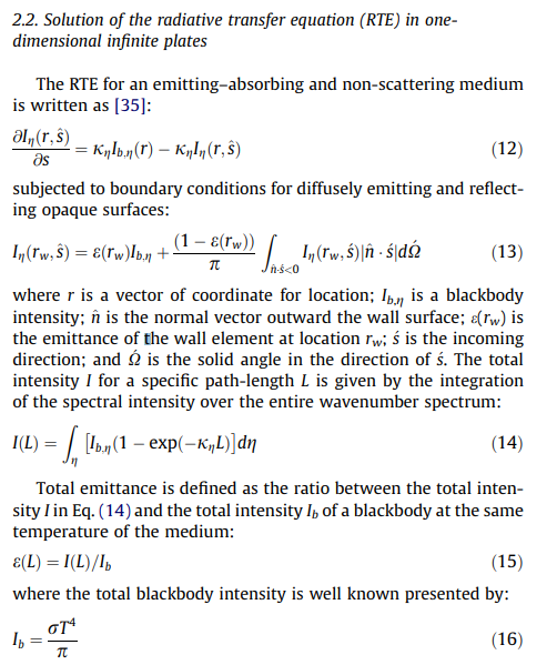
RADIS already computes the spectral absorption coefficients Kappa.
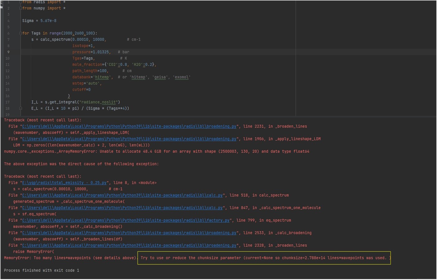
The following quantity in (Eq.14) :
is known as And easily derive the emissivity (Eq.15) . There is also a spectral array called "emissivity_no_slit". Please compare & check, but I think your "emittance"/emissivity above is equal to the integral of the spectral emissivity_no_slit: If you do that, it might be interesting to add a -- PS : the emissivity changes with the path length, but you do not need to recompute the full line-by-line spectrum for each new path length. As long as you already have a computed spectrum at the same temperature, you can rescale the spectrum object (which is really, in RADIS, just an homogenous slab of a given length) which is almost instantaneous, 100% valid and accurate. If you plan to tabulate a database this will save you a lot of time ! There is also a method to rescale mole fraction (i.e, compute the many "MR" of the graph above ) but unlike rescaling path_length, it is strictly speaking not valid as there are 2nd order effects that require to recompute the lineshapes again. If you want to recompute a state-of-the-art database do not use it. However, I'd expect you'd get less than 0.1% error compared to recomputing the line-by-line spectrum from scratch. PPPS : at high pressure (typically >10 atm) a Lorentzian line-by-line model is not valid anymore; you have strong subLorentzian behaviors, and this will change the computed emissivity. Kangwanpongpan's paper does not account for subLorentzian behaviors and it might be partly wrong for the 60+ bars I see being computed . |
|
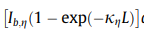
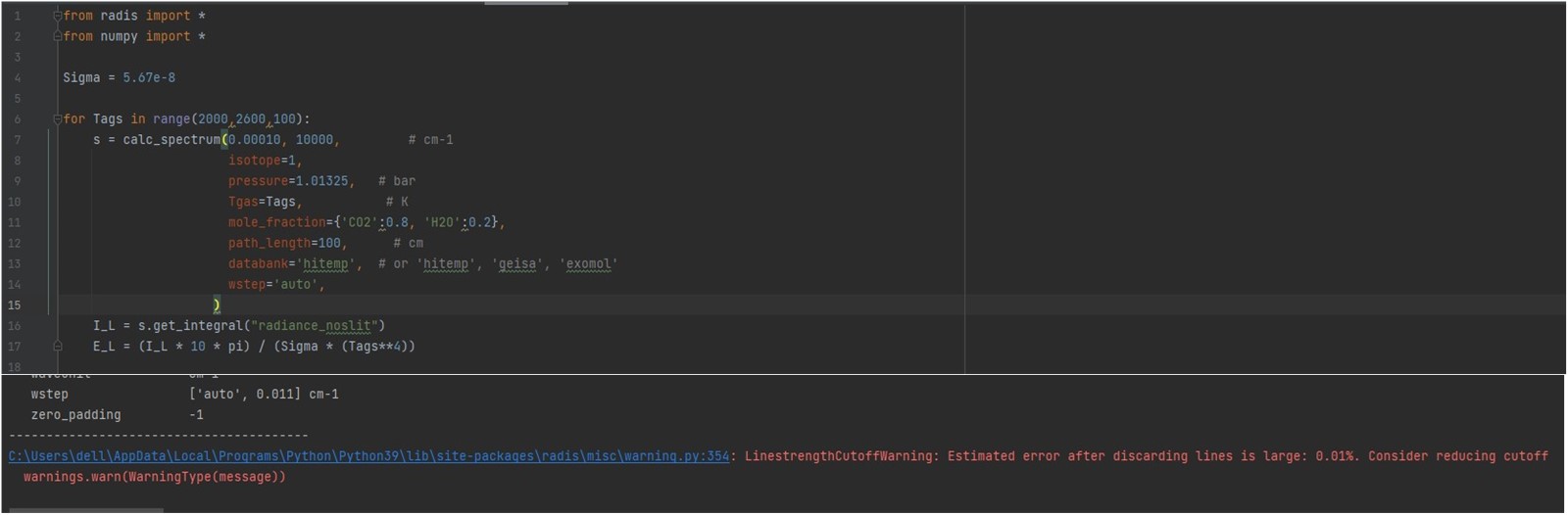
Thanks for the reply Erwan. Your reply helped me a lot and it took me a long time to figure out some of it. I'm new to Radis and relatively new to python, so this could be a silly problem. Now I have a problem, as shown in the figure (shown below). when I calculate the temperature to 2000K, I get an error message, which I solved by reducing the cutoff. After that I ran and got another error message, I don't know how to solve this problem. I would appreciate it if you could answer my question. Thanks very much.
`from radis import * Sigma = 5.67e-8 for Tags in range(300,2600,100): |
|
Memory problem. You're computing extreme amount of lines, which is what you want to do anyway, as I assume you want to compute a reference emissivity database for use in other codes. So expect tens of millions of lines on a spectral grid of hundred-thousands of datapoints. The error message shows you'd need at least 48 GB, therefore a RAM of twice this amount to compute it smoothly. I guess you do not have that available (maybe on a cluster) . You can compute the database over smaller wavenumber ranges, and then join them. There is a Gallery example talking about this ("compute large spectra") You can also increase the wstep parameter. It is currently set to "auto" which ensures a good accuracy, but might be too much in your case. Try 0.01. It will reduce the spectral grid. |
|
#489 was also implemented by @sagarchotalia to help. It cuts the lines in chunks (instead of cutting the wavenumber range), so you don't have to worry about recombining the ranges afterwards. You'd be one of the first users of this feature. No impact on accuracy, but I can't ensure it will be faster than the split-waverange method suggested above. Try! |
|
Thanks for the reply Erwan. I have solved the problem and your reply helped me a lot. Now I calculated a set of data to compare with Kangwanpongpan's paper and found some deviations, especially in the region where the temperature is below 1500K. Is the reason for this deviation what you mentioned before: at high pressure (typically >10 atm) a Lorentzian line-by-line model is not valid anymore; Kangwanpongpan's paper have strong subLorentzian behaviors, and this will change the computed emissivity.
|

|
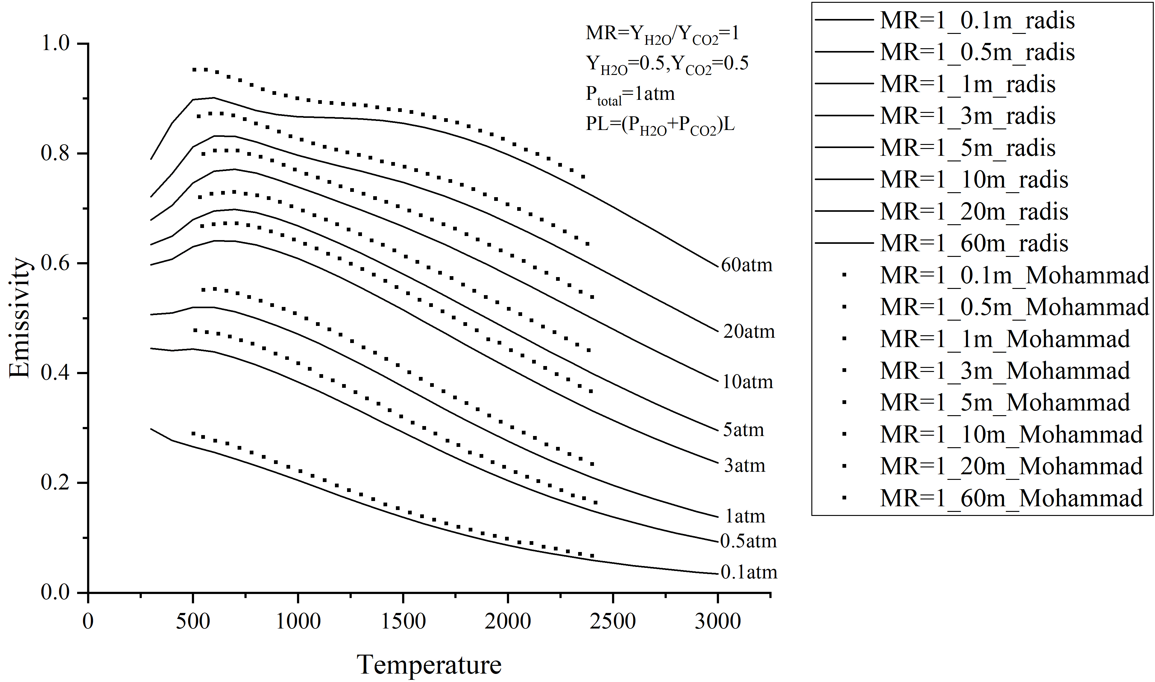
Thanks for the reply Erwan. Now, I have calculated two sets of data using radis, compared with Mohammad Hadi Bordbar's paper and Kangwanpongpan's paper and found some deviations.
I have been thinking about it for a long time but I could not find the reason. I hope you can give some guidance.
|

|
First thing : congratulations for computing all of this!
|
|
Thank you Erwan for your reply, your reply helped me a lot
Sincerely thank you. |
|
Hello I had a quick read at the papers
Their truncatino is based on no physical argument; I assume they just maximized the value until the results made no difference. We know that this is physically wrong : lines are not lorentzian. At least close to ambient temperature & pressure where we have extensive data from the atmosphere communities, we know truncatino should be around 50 cm-1 or (better) use a sub-Lorentzian model directly. See #340 for some calculations on the impact of truncatino. I would : recompute one point using RADIS, for instance near 500 K, 60 atm; using a lineshape Truncation of 500 cm-1. This is not physically accurate but you should match Bordbar result, and confirm that this is the source of the difference. If that's the case, you should defintly publish your paper stating that the differences are due to wrong lineshape models in Bordbar. Truncation half-width is implemented with the If the hypothesis above are correct, Radis model is more accurate (with truncation at 50 cm-1). Better: you should implement some subLorentizan behavior in RADIS ; it would be a first, and who be extremelly accurate. Tagging @mariottop who might be interested in the topic. He might even help you with the paper if needed, emissivity is a strong topic of interest for him. |

|
Hello @PrometheusYao do you have any update ? |
|
@pag1pag you did a similar thing, did you use a dedicated function ? |
🔖 Feature description
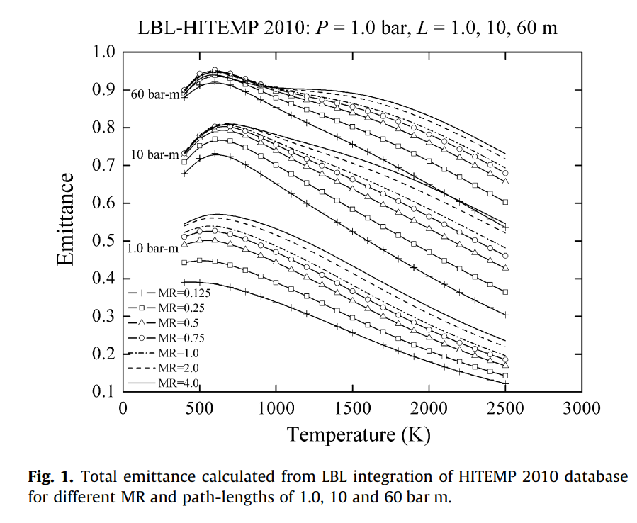
For example this Kangwanpongpan 2012 paper
👉 Why you want this feature!!
No response
The text was updated successfully, but these errors were encountered: