
You can also find all 45 answers here 👉 Devinterview.io - LightGBM
LightGBM (Light Gradient Boosting Machine) is a distributed, high-performance gradient boosting framework designed for speed and efficiency.
- Efficient Edge-Cutting: Uses a leaf-wise tree growth strategy to create faster and more accurate models.
- Distributed Computing: Supports parallel and GPU learning to accelerate training.
- Categorical Feature Support: Optimized for categorical features in data.
- Flexibility: Allows fine-tuning of multiple configurations.
- Speed: LightGBM is considerably faster than traditional boosting methods like XGBoost or GBM.
- Lower Memory Usage: It uses a novel histogram-based algorithm to speed up training and reduce memory overhead.
Traditionally, boosting frameworks employ a level-wise tree growth strategy that expands all leaf nodes on a layer before moving on to the next layer. LightGBM, on the other hand, uses a leaf-wise approach, fully expanding one node at a time, seeking the most optimal split for impurity reduction. This "best-of" procedure can lead to more accurate models but may lead to overfitting if not properly regulated, particularly in shallower trees.
The increase in computational complexity for leaf-wise growth, oft-paramount in models with many leaves or large feature sets, is mitigated by using an approximate method. LightGBM approximates the gain calculation on each leaf, enabling substantial computational savings.
Beyond just the metrics, LightGBM outpaces its counterparts through unique algorithmic techniques. For example, its Split-Finding approach leverages histograms to expedite the locating of optimal binary split points. These histograms compactly encode feature distributions, reducing data read overhead and disk caching requirements.
Because of these performance advantages, LightGBM has become a popular choice in both research and industry, especially when operational speed is a paramount consideration.
LightGBM uses Exclusive Feature Bundling to optimize categorical data, while traditional algorithms, such as XGBoost, generally rely on approaches like one-hot encoding.
-
Binning of Categories: LightGBM bins categorical features, turning them into numerical values.
-
Splits: It can split based on these numerical values, and.
-
Biased Learning: This speeds up learning by favoring frequent categories.
-
One-Hot Encoding: Convert categories into binary vectors where each bit corresponds to a category.
-
Loss of Efficiency: Memory use and computational requirements increase with high-cardinality categorical variables.
Here is the Python code:
import pandas as pd
import xgboost as xgb

data = pd.DataFrame({'category': ['A', 'B', 'C']})
data = pd.get_dummies(data)

# Train XGBoost model
model = xgb.XGBClassifier()
model.fit(data, y)Here is the Python code:
import lightgbm as lgb

data = pd.DataFrame({'category': ['A', 'B', 'C']})

# Train LightGBM model
model = lgb.LGBMClassifier()
model.fit(data, y, categorical_feature='category')Gradient Boosting is an ensemble learning technique that combines the predictions of several weak learners (usually decision trees) into a strong learner.
-
Initial Model Fitting: We start with a simple, single weak learner that best approximates the target. This estimate of the target function is denoted as
$F_0(x)$ . -
Sequential Improvement: The approach then constructs subsequent models (usually trees) to correct the errors of the combined model
$F_m(x)$ from the previous iterations:
where
-
Adding Trees: Each new tree
$h_m(x)$ is fitted on the residuals between the current target and the estimated target, effectively shifting the focus of the model to the remaining errors, making it a Gradient Descent method.
LightGBM employs several strategies that make traditional gradient boosting more efficient and scalable.
-
Histogram-Based Splitting: It groups data into histograms to evaluate potential splits, reducing computational load.
-
Leaf-Wise Tree Growth: Unlike other methods that grow trees level-wise, LightGBM chooses the leaf that leads to the most significant decrease in the loss function.
-
Exclusive Feature Bundling: It groups infrequent features, reducing the search space for optimal tree splits.
-
Gradient-Based One-Side Sampling: It uses only positive (or negative) instances during tree construction, optimizing with minimal data.
-
Efficient Cache Usage: LightGBM optimizes for internal data access, minimizing memory IO.
These combined improvements lead to substantial speed gains during training and prediction, making LightGBM one of the fastest growing machine learning libraries.
LightGBM offers distinct advantages over XGBoost and CatBoost, striking a balance between feature richness and efficiency. Its key strengths lie in handling large datasets, providing faster training speeds, optimizing parameter defaults, and being lightweight for distribution.
- Parallel Learning: Binomial tree grouping algorithm sorts and splits in parallel.
- Sampling: Uses Gradient-based One-Side Sampling (GOSS) and Exclusive Feature Bundling (EFB).
- Loss Function Support: Limited choices like L2, L1, and Poisson, but not advanced ones.
- Categorical Feature Treatment: It handles categoricals with a two-bit approach.
- Missing Data Handling: Methods like
MeanandZeroimputation are primary choices.
- Data Throughput: Utilizes cache more efficiently.
- Parallelism: Employs histogram-based and multi-threading for parallel insights.
- Large Datasets: Pragmatic for extensive, high-dimensional data, and thus ideal for big data scenarios.
- Real-Time Applications: Legendary for swift model generation and inference, crucial for several real-time deployments.
- Resource-Constrained Environments: Its minimal memory requirements mean it's suitable for systems with memory restrictions.
LightGBM leverages exclusive techniques, like leaf-wise tree growth, in bid to ensure accelerated performance and minimal memory requirements.
LightGBM uses a novel leaf-wise tree growth strategy, as opposed to the traditional level-wise approach. This method favors data samples leading to large information gains, promoting more effective trees.
- Concerns: The strategy risks overfitting or ignoring less contributing data.
- Addressed: LightGBM features mechanisms like
max-depthcontrol, minimum data points needed for a split, and leaf-wise technique subsampling.
This technique maximizes resource usage by selecting data points offering most information gain potential for updates during tree building, especially when dealing with huge datasets.
- Process: LightGBM sorts data points via gradients, then utilizes a user-specified fraction with the most significant gradients for refinement.
LightGBM facilitates quicker examination of categorical features by sorting and clustering distinct categories together, enhancing computational efficiency.
The framework ensures simplicity and independence of computation across tree nodes, heightening feature parallelism.
LightGBM can still deliver remarkable training speed on a CPU, especially for sizeable datasets, using its core strategies without necessitating a GPU.
The histogram-based approach, often called "Histograms for Efficient Decision Tree Learning," is a key feature in LightGBM, a high-performance gradient boosting framework.
This method makes training faster and more memory-efficient by bypassing the need for sorting feature values during each split point search within decision trees.
LightGBM employs the Gradient-Based One-Side Sampling (GOSS) algorithm to choose the optimal splitting point. This method focuses on the features that most effectively decrease the loss, reducing computations and memory usage.
- Top-K: Select a subset of the instances with the largest gradients.
- Random Unselected: Combine some remaining instances randomly.
- Sort Features: Rank features by their relevance.
- Incidence Index: Calculate the on-going loss for each split point candidate.
- Best Split: Determine the point that yields the most significant loss reduction.
# Reducing gradients and instance count
goss_topk = np.argsort(gradient)[:k]
goss_random_unselected = np.random.choice(
    np.setdiff1d(np.arange(n_instances), goss_topk), size=n_selected-k)

# Computing gradients' threshold
grad_threshold = np.percentile(gradient[goss_topk], 90)
goss_topk = goss_topk[gradient[goss_topk] >= grad_threshold]

# Selecting the best split
best_split = np.argmin(loss[goss_topk])To prepare data for the histogram-based method, features are divided into equally spaced bins. Each bin then covers a range of feature values, making the computation more efficient.
# Original feature values
feature_values = [1, 5, 3, 9, 2, 7]

# Binning with 2 bins
bin_edges = np.linspace(min(feature_values), max(feature_values), num=3)
binned_features = np.digitize(feature_values, bin_edges)The algorithm builds a histogram for each feature, where the bin values represent the sum of gradients for instances falling into that particular bin.
# Gradients
grad = [0.2, -0.1, 0.5, -0.4, 0.3, -0.2]

# Histogram with 2 bins
histogram = [np.sum(grad[binned_features == b]) for b in range(1, 3)]The Gain-Based Split Finding algorithm evaluates each potential split point's gain in loss function to select the optimal one.
The histogram-based approach significantly reduces the computational and memory requirements compared to the traditional sorting-based methods, particularly when the dataset is larger or the number of features is substantial.
LightGBM offers two tree-growth methods: leaf-wise (best-first) and depth-wise (level-wise). Let's look at the strengths and limitations of each.
Leaf-wise growth updates nodes that result in the greatest information gain. The benefits of this method include:
- Potential Speed: Leaf-wise growth can be faster, especially with large, sparse datasets where there might be insignificant or no information gain for many nodes.
- Overfitting Risk: Without proper constraints, this method can lead to overfitting, particularly on smaller datasets.
Depth-wise tree growth, often referred to as level-wise growth, expands all nodes in a level without prioritizing the ones with maximum information gain. The method has these characteristics:
- Overfitting Control: Because depth-wise growth divides forests using fixed-depth trees, it generally helps to prevent overfitting.
- Training Speed: For dense or smaller datasets, it can be slower than leaf-wise growth.
8. What is meant by "leaf-wise" tree growth in LightGBM, and how is it different from "depth-wise" growth?
In LightGBM, the term "leaf-wise" refers to a specific strategy for tree growth. This approach differs fundamentally from the more traditional "level-wise" (also known as "breadth-first") strategy regarding the sequence in which nodes and leaf nodes are expanded.
In traditional decision trees, such as in the case of HistGradientBoosting algorithm, trees are typically grown level by level. This means that all nodes at a given depth are expanded before moving on to the next depth level. All leaf nodes at one depth level are generated before any nodes at the next depth level.
For example, consider the following sequence when growing a tree:
- Expand the root
- Expand depth 1 nodes
- node 1
- node 2
- Expand depth 2 nodes
- node 3
- node 4
- node 5
- node 6
Here, the nodes are expanded one after the other.
The "leaf-wise" method, in contrast, is an approach to tree building where nodes are grown by optimizing based on the projected gain up to the next best leaf node. This implies that the model may prioritize a node for splitting if stopping criteria are satisfied prior to fully expanding its parent nodes. Consequently, under this strategy, different nodes can have varied depths.
LightGBM's default configuration uses the "leaf-wise" approach to maximize tree leaf-wise potential function. However, this method may lead to over-fitting in some cases, especially when used with smaller datasets, and it is recommended to use it in conjunction with max_depth and min_child_samples.
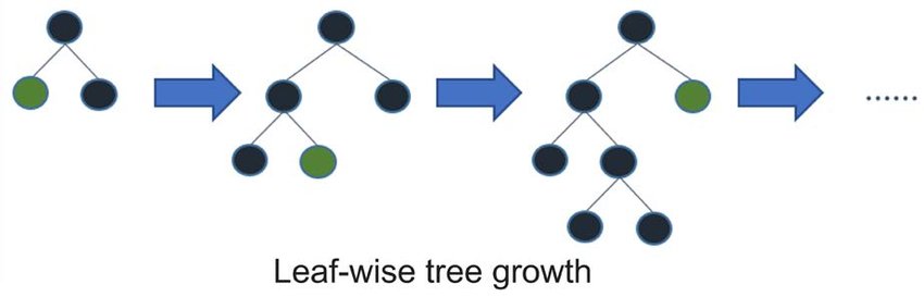
The image link to "Leaf Wise Trees" can also be found in the research paper "LightGBM: A Highly Efficient Gradient Boosting Decision Tree" by Microsoft.
For improved precision and speed, LightGBM incorporates two techniques in conjunction with its leaf-wise growth:
- Gradient-based One-Side Sampling: Focuses on observations with larger gradients when considering those eligible for tree partitioning.
- Exclusive Feature Bundling: Minimizes memory utilization and computational expenses by integrating exclusive features into the same bins.
- Improved Accuracy: Leaf-wise growth can identify more predictive nodes.
- Faster Performance: By focusing on the nodes with the highest information gain, the tree development process is streamlined.
- Overfitting Risk: The approach might lead to overfitting, notably in datasets with limited samples.
- Memory Utilization: Leaf-wise growth can use more memory resources, particularly with substantial datasets.
LightGBM addresses overfitting using an approach unique to its architecture. By leveraging both regularization techniques and specialized splitting methods, it effectively minimizes these risks.
-
Max Delta Step: Also known as "maximum difference allowed,"
$\delta$ , this mechanism constrains the updates made to the leaf values, mitigating overfitting by avoiding steep changes. -
XGBoost-like Constraints: LightGBM shares parameters with XGBoost, such as max depth and min data in leaf, to exercise control over tree growth.
-
Bagging: Also known as
repeated subsampling, LightGBM randomly selects a subset of data for tree construction. This technique emulates the "forest" in "random forest," reducing overfitting by introducing variety among trees. -
Bounded Split Value: LightGBM limits the range wherein it considers a feature's split points, based on quantiles. This strategy shuns overfitting by focusing on more stable points for the split.
-
Early Stopping: Through periodic validation evaluation, LightGBM can terminate model training, arresting overfitting when the validation metrics start to degrade.
-
Leaf-wise Tree Construction: By building trees in a "leaf-wise" fashion, LightGBM prioritizes the branches that yield the most immediate gain.
-
Post-Pruning: The framework employs a variation of post-trigger light top-down global binary tree reduction, which helps "prune" the tree of insignificantly contributing nodes.
-
Categorical Feature Support: For categorical features, LightGBM applies a specialized algorithm, the "DType" algorithm, to enhance performance and diminish model complexity.
-
Improved Feature Fraction Handling: LightGBM's enhanced feature fraction mechanism further dampens the risk of overfitting.
-
Exclusive Feature Bundles: Utilizing in-built routines, LightGBM can discern an optimal combination of features that enhances generalization.
-
Rate-Monitored Learning: By gauging the learning rate, the model stays on course, avoiding rapid or over-vigorous updates.
-
Continuous Validation: Through continuous validation, akin to 'n-fold cross-validation', LightGBM can gauge out-of-sample performance at each training interval, combating overfitting behaviors.
-
Hessian-Aware Split Evaluation: Incorporating Hessian (second-order derivative) in split evaluations turns LightGBM into a more "sensitive" learner, adept at steering clear of overfitting vulnerabilities.
LightGBM offers stochastic gradient boosting (SGB) and dropouts, two proven techniques that arrest overfitting with ease. The toolset is armed with benchmarking mechanisms that accurately compute optimal dropout probabilities, enriching the model's protective shell.
- L1 (Lasso): By favoring models with fewer, non-zero weighted features, L1 helps stop overfitting.
- L2 (Ridge): Encouraging balance, L2 regularization ensures all features play their part, thwarting dominance by a select few.
Both these regularizers necessitate a penalty coefficient, designated as
LightGBM does not shy away from the incorporating advanced ensemble techniques, such as 'secondary constraints' by building sub-models at certain training phases to strengthen models' defenses against overfitting.
When you are unsure of the best method in your business, cross-validation (CV) is typically the gold standard. Both LightGBM and XGBoost offer functionalities for automatic cross-validation, but LightGBM also proposes a manual trial if you have the specifics in mind. Whether you pick stratified or time-based CV, LightGBM facilitates a range of split-generating tools, allowing you a plethora of setups to test out.
Ultimately, as the safeguarding procedures underline, LightGBM is a trailblazer, aggressively innovative in battling overfitting and never ceased in its orientation toward best-in-class predictive consistency.
Feature Parallelism and Data Parallelism are key techniques employed by LightGBM for efficient distributed model training.
In the context of LightGBM, Feature Parallelism entails distributing different features of a dataset across computational resources. This results in parallelized feature computation. LightGBM splits dataset columns (features) and subsequently evaluates feature histograms independently for each subset.
The process involves the following main steps:
- Column Partitioning: Features are divided or partitioned into smaller groups (e.g., 10 feature groups).
- Histogram Aggregation: Each partitioned feature group is used to compute histograms which are then merged with histograms from other groups.
- Histogram Optimization: For dense features or specific hardware configurations, sorted histograms can be utilized. Advises on the histogram types to use. This approach effectively reduces computation needs and is especially useful when device memory or CPU capacity is limited.
In LightGBM, Data Parallelism operates at the level of individual training instances (rows) in a dataset. It involves distributing different subsets of the dataset to different computational resources, causing parallelized tree building across the resources.
LightGBM employs a sorted data format, where the dataset is continually re-organized based on the feature that provides the best split. This is referred to as the feature for the current node in the ongoing tree induction process.
LightGBM isn't bound to orthogonality between the techniques. It skillfully merges both Feature and Data parallelism.
11. How do Gradient-based One-Side Sampling (GOSS) and Exclusive Feature Bundling (EFB) contribute to LightGBM's performance?
Gradient-based One-Side Sampling (GOSS) and Exclusive Feature Bundling (EFB) are two key techniques that contribute to the efficient and high-performance operation of LightGBM.
-
GOSS for targeted data sampling: The method employs full sets of data points for the strong learners, reducing the amount when training weak learners. This selective sampling leads to a performance improvement seen in Categorical and High-Cardinality Features.
-
EFB enhances feature bundling: Utilized with LightGBM's exclusive leaf-wise tree growth, EFB increases the granularity of feature bundles. The technique is especially effective in case the dataset entails Unique Identifiers.
-
EFB minimizes computational load: With a focused selection of features, EFB optimizes memory and CPU resource utilization. This makes it ideal when working with Large Datasets, conserving both processing time and hardware requirements.
Here is the Python Code:
import lightgbm as lgb

# Enable EFB
params = {
    'feature_pre_filter': False,
    'num_class': 3,
    'boosting_type': 'gbdt',
    'is_unbalance': 'true',
    'feature_fraction': 1.0,
    'bagging_fraction': 1.0
}
lgb.Dataset(data, label_label, params=params, free_raw_data=False).construct()In the LightGBM algorithm, the learning rate (LR), also known as shrinkage, controls the step size taken during gradient descent. Setting a proper learning rate is key to achieving optimal model performance and training efficiency.
-
Convergence Speed: A higher learning rate leads to faster convergence, but the process can miss the global minimum. A lower rate might be slower but more accurate.
-
Minimum Search: By regulating the step size, the learning rate helps the model in finding the global minimum in the loss function.
-
Shrinkage Rate: Defined as
learning_rate, it sets the fraction of the gradient to be utilized in updating the weights during each boosting iteration. -
Regularization Parameters: Learning rate is linked to the use of other parameters such as L1 and L2 regularization.
Here is the Python code:
import lightgbm as lgb

# Initializing a basic model
model = lgb.LGBMClassifier()

# Setting learning rate
params = {'learning_rate': 0.1, 'num_leaves': 31, 'objective': 'binary'}LightGBM, a popular tree-based ensemble model, offers some unique hyperparameters to optimize its tree structure.
When fine-tuning the number of leaves or the maximum tree depth, here are some of the key considerations.
- Intended Use: Specifies the maximum number of leaves in each tree.
- Default Value:
$31$ . - Range:
$>1$ . - Impact on Training: Highly influential, as more leaves can capture more intricate patterns but might lead to overfitting.
- Intended Use: Defines the maximum tree depth. If set,
num_leavesconstraints become loose. - Default Value:
$6$ . - Range:
$>0$ or$0$ , where$0$ suggests no constriction. - Impact on Training: Higher depth means trees can model more intricate relationships, potentially leading to overfitting.
-
Start with Defaults: For many problems, default settings are a good initial point as they are carefully chosen.
-
Exploratory K-Fold Cross-Validation: Assessing performance across different parameter combinations provides insights. For
num_leavesandmax_depth, consider- Grid Search: A systematic search over ranges.
- Random Search: Pseudo-random hyperparameter combinations allow broader exploration.
- Bayesian Optimization: A smarter tuning strategy that adapts based on past evaluations.
- Metrics: Both classification and regression tasks benefit from rigorous tuning. Common metrics, such as AUC-ROC for classification and Mean Squared Error for regression, guide parameter selection.
- Speed-tradeoff: LightGBM's competitive edge comes from its efficiency. Larger leaf or depth configurations can slow down training and might be less beneficial.
Emphasizing adaptability and the ability to learn from your iterative tuning experiences.
In LightGBM, the min_data_in_leaf parameter controls the minimal number of data points in a leaf node. The greater the value, the more conservative the model will be, experiencing reduced sensitivity to noisy data.
-
IDX Splitting: Used for two-class or exclusive multi-class classification, it halts leaf-wise growth when the values in a leaf become unbalanced. Balanced leaf nodes can curb overfitting.
-
Exclusive Feature Bundling: Applies to exclusive multi-class problems. A small leaf imbalance is tolerated if one of the chosen features is exclusively advantageous for one class.
-
Bidirectional Splitting: Utilized for regression tasks, it can split along either direction of a feature's gradient, moderating overfitting.
-
Data Consistency: On consistent datasets, increasing
min_data_in_leafmight heighten model robustness. With varied datasets, it could lead to inferior outcomes. -
Regularization through Ensembling: By promoting broader splits and restraining the depth of the tree, it can shrink the number of trees the model builds. Consequently, ensemble methods like bagging and early-stopping could prove less necessary.
-
Fast Deployment: For rapid model integration, utilize larger
min_data_in_leafvalues, thus streamlining the model tree structure. -
Less Noisy Outcomes: Discard extraneous noise by opting for a stricter splitting criterion.
-
Resource Efficiency: With fewer leaf nodes requiring examination, prediction speed elevates.
-
Customized Model Building: Influence the model's behavior based on the nature of your dataset: use smaller values for noise-free datasets and larger ones for noisier ones.
The bagging_fraction parameter in LightGBM determines the subset size of data for each boosting iteration. This can have a substantial impact on model characteristics.
- Higher Variance: The model becomes sensitive to the specific subset of data used for training in each boosting round, potentially leading to higher variability in predictions.
- Increased Risk of Overfitting: With more noisy data being included, the model may fit better to the training data but potentially at the cost of increased overfitting to noise.
- Faster Training: Using a smaller subset of data can speed up the training process as fewer instances need to be processed in each boosting round.
- Lower Variance: By training on more diverse sets of data, the model becomes more robust and generally leads to more stable predictions.
- Reduced Risk of Overfitting: Including a higher fraction of the dataset can mitigate overfitting, especially in settings where the number of samples is small.
- Slower Training: As it's training on a larger dataset in each boosting round, it will be slower compared to using a smaller subset.
The choice of bagging_fraction should be guided by, among other factors, the trade-off between overfitting and computational efficiency. LightGBM's early stopping mechanism and cross-validation can help determine the optimal bagging_fraction for a given dataset and task.
Explore all 45 answers here 👉 Devinterview.io - LightGBM