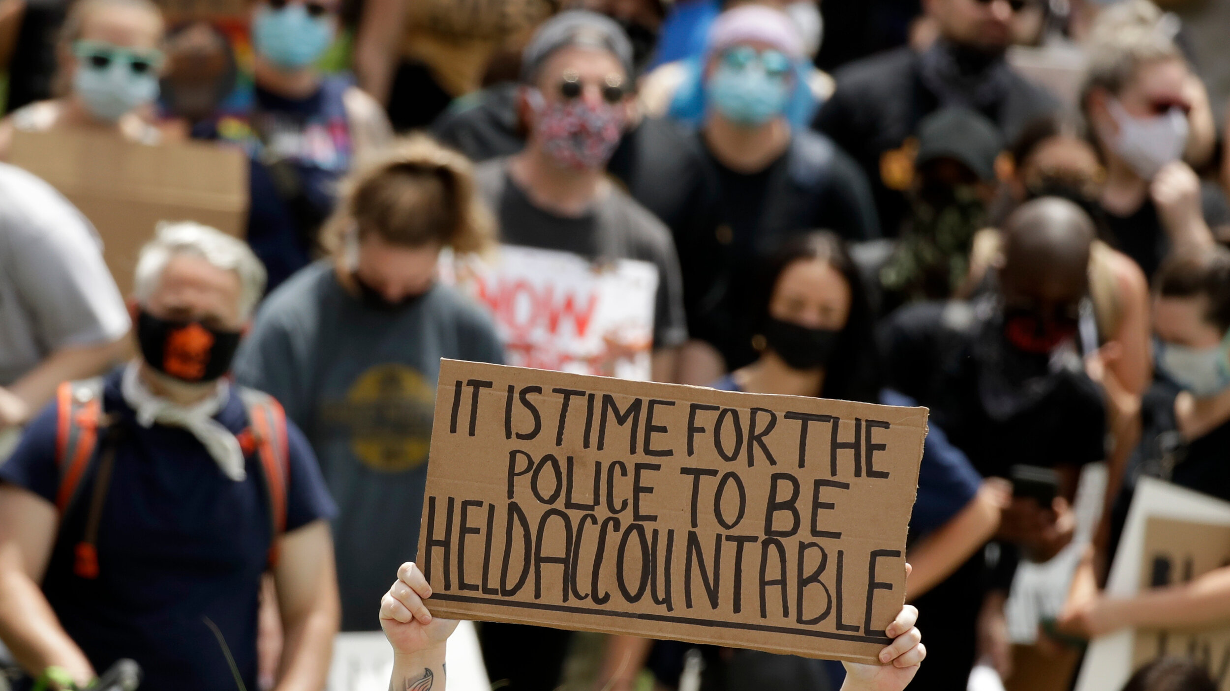
From Rodney King to Trayvon Martin to Ma'Khia Bryant: the police violence against civilians in the United States is a fact, a significant socio-political challenge and a major human tragedy. In 2020, when one of the four police officers at the scene murdered a black American man George Floyd by kneeling on his neck for 9 minutes and 29 seconds, Floyd's last words 'I can't breath' became a slogan that lead to mass uprising in the US and across the world. Yet, since the arrest of his murderer Derek Chauvin, at least 3 people were killed by the police every day.
This project intends to analyze police violence (while police violence can be interpeted in various ways, in this instance we are recording only fatal for the civilians encounters with the law enforcement) across the United States in 2013-2020, detect the states where the police is more prone to violence and analyze whether there is racial and/ or other bias in violent police behavior. The project is also looking to compare the budgets of the police departments in the states where police violence is at highest. Among other things the project is looking at: correlation between the age of the victims and whether they attempted to flee the scene; comparisons between US population by race and US police victims by race. For a brief project review, refer to the project presentation slides. For a more detailed outline continue reading below.
The project research is focused around the following questions:
- WHAT ARE THE TOP STATES/ COUNTIES FOR POLICE VIOLENCE IN 2013-2020?
- WHAT IS THE DEATHS BREAKDOWN BY RACE VS. COUNTRY POPULATION BY RACE?
- IS THERE A CORRELATION BETWEEN THR AGE OF TH VICTIM AND WHETHER THEY FLED?
- WHAT ARE THE POLICE DEPARTMENTS' BUDGETS?
- CAN POLICE VIOLENCE IN THE US BE PREDICTED BASED ON FACTORS SUCH AS RACE?
The project has used the Police Killings in 2013-2020 dataset as the main resource. Below are some of the supporting datasets that the project has also leaned on:
- Police Stations/ Departments Budgets
- Washington Post Police Shooting Data 2015-2021
- Kaggle Datasets on Police Violence and racial Equity
The project has used the following documentation tools:
- Pandas Categorical Data
- Seaborn Documentation
- imbalanced-learn documentation
- scikit-learn documentation
- Jupyter Notebook
- Python v3.x
- Pandas
- Numpy
- Seaborn
- Matplotlib
- SciKit-Learn
- Imbalanced-Learn
- SQLAlchemy
- MySQL
- JSON
- Pyscopg2
- Database: The project used Postgres SQL and Python Pandas were used to load, clean and analyze the data (for data loading documentation refer here, including the ERD.
- Host Instance: The project data is stored in AWS RDS.
- Machine Learning (Python): The project used SciKitLearn to create and test the machine learning (ML) model. The ML model is testing a predictive statistic (For further details please refer here).
- Visualization: The project used visuals from the ML analysis as well as Tableau to visualize the analysis. Data is visualized in a simplified manner for all stakeholders to be able to access the validity of it. Data is presented in a story format (To review the dashboard in Tableau please refer here).
To answer the listed above questions the project team reviewed the datasets listed previously, selected the main and the supporting datasets, and worked on cleaning and analyzing them. The main dataset was preprocessed and analyzed in order to test a few ML models and to select the most appropriate one. The supporting datasets helped inform and complete the visual analysis that was performed in Tableau.
The police violence data set was imported from AWS into a Pandas DataFrame. The DataFrame originally contained 20 columns and 9,082 rows of data. Column names include: Victim_Age, Victim_Gender, Victim_Race, Date, City, State, County, Responsible_Agency, Cause_of_Death, Brief_Description, Criminal_Charges, Mental_Illness, Armed_Status, Threat_Level, Fleeing, Body_Camera, Geography, Encounter_Type, Initial_Reason_for_Encounter, and Call_for_Service.
Victim_Gender, City, State, Criminal_Charges, and Brief_Description were dropped since they were not going to be used in the model prediction.
The DataFrame was inspected for null values and any columns with 2,000 or more null values were filled in with a variable. The decision to fill in null values was made because if all rows with null values were dropped, it would significantly affect the data set. The variables used to fill in null values were ones that were already found in the column. The following columns were had null values replaced with a variable: Threat_Level, Fleeing, Body_Camera, Encounter_Type, Initia_Reason_for_Encounter, and Call_for_Service.
Columns that contained 70 or less null values had their rows dropped.
The data type for the Victim_Age column was converted from an object to an integer because this feature needed to be an integer.
Additional columns from the Date column were created. New columns created include Day, Month, Year, Day_of_the_Week, and Holiday. This data may be used to predict when some is more likely to be killed by law enforcement. The Date column was dropped because it was no longer needed once Day, Month, Year, Day_of_the_Week, and Holiday were extracted from it.
Counts of Victim_Race were also calculated:

Lastly, the Victim_Race values were converted to numbers:

Data was trained and tested on police_killings database that was stored in AWS. This database was comprised of data from The Washington Post and Kaggle.
The AWS police_killings database was split into a training and testing data set. The training data set was made up of 8 rows and 5,995 columns. This will be the data the model learns from.
The test data set consists of the remaining data and will be used to assess the model's performance.
The following columns were transformed into numerical values using the get_dummies method: Cause_of_Death, Mental_Illness, Armed_Status, Threat_Level, Fleeing, Body_Camera, Geography, County, Responsible_Agency, Encounter_Type, Intitial_Reason_for_Encounter, and Call_for_Service. These will were the features the model trained on.
The column Victim_Race was dropped because this is the target variable that will be used to predict the outcome.
Random Forest, Decision Tree, and Logistic Regression models were tested. Note that none of the models were optimized at this time. Overall, all three models performed relatively the same, but future progress on this model will use Random Forest. Results below are of the initial tests of the models.
Random Forest is a supervised machine learning algorithm that creates decision trees on randomly selected data samples, gets predictions from each tree and selects the best solution by means of voting. The prediction result with the most votes is selected as the final prediction.
Random Forest gave the following scores:
Receiver Operator Characteristic — Area Under the Curve (ROC AUC) score: 0.565

The ROC AUC score for this model means that 56.5% of classes are correct and 43.5% are incorrect.
An average precision score of 0.53 means that this model predicted positive class predictions 53% of the time.
An average recall score of 0.53 means that 53% of class predictions made out of all positive examples in the dataset were correct and 47% were incorrect.
Decision Tree is another supervised machine learning algorithm that can make predictions by learning simple decision rules inferred from test data.
Decision Tree gave the following scores: ROC AUC: 0.561

The ROC AUC score for this model means that 56.1% of classes are correct and 43.9% are incorrect.
An average precision score of 0.53 means that this model predicted positive class predictions 53% of the time.
An average recall score of 0.53 means that 53% of class predictions made out of all positive examples in the dataset were correct and 47% were incorrect.
Logisitc Regression is a supervised machine learning algorithm that is used to assign observations to a discrete set of classes.
Logistic Regression gave the following scores: ROC AUC: 0.516

The ROC AUC score for this model means that 51.6% of classes are correct and 48.4% are incorrect.
An average precision score of 0.30 means that this model predicited positive class predictions 30% of the time.
An average recall score of 0.46 means that 46% of class predicitions made out of all positive examples in the dataset were correct and 54% were incorrect.
- Random Forest requires a lot of time and computational power. The large number of trees can make the algorithm too slow and ineffective for real-time predictions. A more accurate prediction requires more trees, which results in a slower model.
- Due to the ensemble of decision trees, it can suffer interpretability and fails to determine the significance of each variable.
- Random Forest prevents overfitting by creating trees on random subset.
- Random forest adds additional randomness to the model, while growing the trees. Instead of searching for the most important feature while splitting a node, it searches for the best feature among a random subset of features. This results in a wide diversity that generally results in a better model.
- It automates missing values present in the data.
- Normalising of data is not required as it uses a rule-based approach.
The police killings dataset originally consisted of 16 columns and 9,082 rows of data:

In order to begin training the model several columns were encoded using the get_dummies() method.
killings_encoded = pd.get_dummies(killings_df, columns =
                                  ['Cause_of_Death', 'Mental_Illness', 'Armed_Status', 'Threat_Level', 'Fleeing',
                                   'Body_Camera', 'Geography', 'County', 'Responsible_Agency', 'Encounter_Type',
                                   'Initial_Reason_for_Encounter', 'Call_for_Service'])
The Victim_Race column in the data set contained the following counts of races:
White 3935 Black 2259 Hispanic 1566 Unknown Race 903 Asian 134 Native American 127 Pacific Islander 50
The features were created by dropping the Victim_Race column and using get_dummies() on the remaining columns. Victim_Race was the target values.
The dimensionality method of Principal Component Analysis (PCA) was used in order to reduce the size of the data set by transforming the large number of variables into a smaller one that still contained most of the information in the original data set. The trade-off with using PCA is accuracy, but the trade-off is simplicity.
The model was fitted and transformed with 30% of the original data. PCA computes a new set of variables (principal components) and expresses the data in terms of these new variables. The new variables represent the same amount of information as the original variables and the total variance remains the same.
The model was then trained, tested, and split with the new DataFrame created by PCA. Stratify was also used with train_test_split in order to make the target more evenly distributed.
The model was fitted with the Random Forest algorithm. The model gave a ROC accuracy score of .610, or 61%.
The classification report is as follows:

The races White (1), Black (2), and Hispanic (3) had precision scores of 0.59, 0.54, and 0.57, respectively. This means that the model made positive class predictions 59%, 54%, and 57% of the time. The Random Forest model made positive class predictions for races Unknown (4), Asian (5), Native American (6) 33% of the time and 83% of the time for Pacific Islander (7).
The overall precision average of this model is 54%.
Recall is the number of members of a class that the model identified correctly divided by the total number of members in that class. The model correctly identified the races White (1) 88% of the time, followed by Black (2) at 44%, and Hispanic (3) at 39%. The races Unknown (4), Asian (5), Native American (6), and Pacific Islander (7) had recall scores of 4%, 3%, 3%, and 42%, respectively.
The overall recall score of this model is 57%.
The confusion matrix is used to express how many of this model's predictions were correct, and when incorrect, where the model got confused. The rows represent true labels and the columns represent predicted labels. Values on the diagonal represent the number (percentage) of times where the predicted label matched the true label (same as recall). Values in the other cells represent instances where the model mislabeled an observation, so the columns displays what the classifier predicted, and the row displays what the correct label was. This provides an easy way to see where the model may need additional training.

An attempt was made to optimize this model using hyperparameterization, which is like adjusting the settings of an algorithm. For Random Forest models, hyperparameters include the number of decision trees in the forest and the number of features considered by each tree when splitting a node. This is usually a trial-and-error process.
This process can make a model prone to overfitting, so in order to combat that, the technique of Cross Validation (CV) was employed. The method K-Fold CV was used, which further splits the training set into K number of subsets, which are known as 'folds'. The model is then fit K times, and each time time the model is trained on K-1 (K minus 1) of the folds and evaluated on the Kth fold, which is the validation data.
The following parameters were used on the Random Forest Model
param_grid = {
    'max_depth': [10, 20, 50],
    'max_leaf_nodes': [10],
    'n_estimators': [100],
'max_features': [10]- max_depth is the max number of level in each decision tree, so the parameters of 10, 20, and 50 are the depth of the decision tree levels
- max_leaf_nodes grows the tree in best-first fashion until max_leaf_nodes are reached
- n_estimators is the number of trees in the forest
- max_features is the maximum number of features considered for splitting a node
This set of parameters fit 3 folds for each of the 3 candidates, for a total of 9 fits.
The Random Forest model was then re-fit with these new parameters. Its ROC accuracy score was 0.620, or 62%, which is slightly better than the original model.
The classification report is as follows:

The races White (1), Black (2), and Hispanic (3) had precision scores of 0.59, 0.53, and 0.53, respectively. This means that the model made positive class predictions 59%, 53%, and 53% of the time. The Random Forest model made positive class predictions for races Unknown (4) 38% of the time, Asian (5) 100% of the time, Native American (6) 75% of the time, and 75% of the time for Pacific Islander (7).
The overall precision average of this model is 55%, which is not much, but predictions improved for several of the races. The precision for Unknown improved by 5%, Asian improved by 17%, Native American improved by 42%, and Pacific Islander improved by 8%.
The average recall score of the optimized Random Forest model is 57%, which is the same as the previous model; however, some of the scores for the individual races changed.
The recall scores for Black, Unknown, and Asian did not change.
White had a decrease in recall score from 88% to 86%.
The following races showed improvements in their recall scores:
- Hispanic - 39% --> 40%
- Native American - 3% --> 9%
- Pacific Islander - 42% --> 50%
The confusion matrix for the optimized model:

The datasets don't differentiate between civilian victims that were killed at a crime scene and during random encounters with the police (such as during a routine traffic stop). The budgets dataset only goes until 2017, therefore the project team cannot perform the correlation analysis for the 2017-2020 years between the killings and the budgets.
As some of the post-bootcamp steps the project considers to compare the US police stations data in terms of budgets, training and arming/ disarming the police officers with other countries, including those countries where the police don't carry arms.We also would need to continue working on PCA and tuning hyperparameters. The goal is to retain over 80% of the data/information contained in the original data set.

- Phoenix, AZ is the state with the most number of police killing. Phoenix has a black population of 6.5% but 15% of police killing were black.
- From 2013-2020, 25% the victims of police killings where black. This number isn't consistent with the overall population of blacks in the US.
- Based on the total amount police killings 43% of victims weren’t fleeing, 32% of victims were unknown, 11% fled by car, 9% fled on foot, and 5% used other methods. Age isn’t a factor because ‘not fleeing’ and ‘unknown’ have the highest percentage in almost all age ranges.
- There is no clear correlation between police department budgets and the amount of police killings. Los Angeles, CA and Phoenix, AZ had 125 and 131 police killings respectfully. Los Angeles had a budget that was $271.77 million more.
- At this time, model predictions are skewed. Further tuning and optimization is needed in order to make a reliable prediction on activities will most likely lead to the victim getting killed.