ww_tvol_study

Code and results of Hugonnet et al. (2021), Accelerated global glacier mass loss in the early twenty-first century. 🌎 ❄️

Below a short guide to: manipulate the dataset, reproduce the processing steps, and reproduce the figures and tables.

Manipulate the dataset

Retrieve the data

The dataset consists of:

1. Cumulative time series of volume and mass change (.csv, ~500MB) at an annual time step and rates of volume and mass changes (.csv, ~3GB) for successive 1-, 2-, 4-, 5-, 10- and 20-year periods of 2000-2019, both for global, regional (RGI O1 and O2), per-tile (0.5x0.5°, 1x1° and 2x2°) and per-glacier, available at https://doi.org/10.6096/13.
2. Elevation change rasters (.tif, ~15GB) at 100 m posting for successive 5-, 10- and 20-year periods of 2000-2019, available at https://doi.org/10.6096/13.
3. Elevation time series (.nc, ~3TB) at 100 m posting and monthly time step, only available on-demand (see note below).
4. Bias-corrected ASTER DEMs (.tif, ~10TB) at 30 m posting, only available on-demand (see note below).

Important note for data only available on-demand (3. and 4.): This data is very large (several TBs) and, in the case of ASTER DEMs, unfiltered (for artefacts, clouds, etc). It is very difficult to use. If that is nonetheless needed, contact me with latitude-longitude coordinates of your area of interest, and a description of your intended use.

Other notes:

• Global and regional series of specific (area-scaled) change presented throughout the article (e.g., mean elevation change) use estimates of time-varying glacier areas (see Methods). Due to the lack of such estimates per individual glaciers, specific change per glacier is computed with fixed areas. This means that only global and regional direct mass/volume change are consistent with the individual glacier contributions of a given region.
• Cumulative mass change series and rates for periods shorter than 5 years are provided, but do not respect assumptions of density conversion of Huss (2013), possibly resulting in too small uncertainties.
• Rates uncertainties over a specific period (e.g., 2004-2011) need to be derived from the cumulative volume change time series, due to the varying spatial correlation at each point in time (volume time series) and temporal correlation at the regional scale assumed for certain uncertainties (density conversion).
• Tile mass changes (e.g., 1x1° grid) currently rely on per-glacier integrated volumes, aggregated according to glacier outline centroids. Therefore, those changes are not necessarily representative of mass change within the exact spatial boundaries of the tile. Deriving such changes is more complex and is not available yet (contact me for more details).

Setup environment

Most scripts rely on code assembled in the packages pyddem (DEM time series) and pymmaster (ASTER processing), which themselves are based on pybob (GDAL/OGR-based georeferenced processing).

You can rapidly install a working environment containing all those packages and their dependencies with the ww_tvol_env.yml file, located at the root of the repository, using mamba:

mamba env create -f ww_tvol_env.yml

Important note: for pybob, the development branch installed by the environment file to work with this repository is iamdonovan/test_dev and not the main branch.

Further details on setup and functions present in these packages are available through pyddem documentation and pymmaster documentation.

How to use

Scripts for selecting or manipulating the dataset at various scales are located in dataset/ and divide in three sections:

• gla_vol_time_series/ for the volume and mass change time series integrated over glaciers (.csv),

• h_time_series/ for the elevation time series and elevation change rasters (.nc and .tif),

• raw_dems/ for the bias-corrected ASTER DEMs.

Below a few examples:

import pyddem.tdem_tools as tt
import pyddem.fit_tools as ft
import numpy as np
# filename of file containing RGI 6.0 metadata (updated for some regions in this study) for all glaciers
fn_base = '/path/to/base_rgi.csv'
# filename of file containing our estimates for all glaciers
fn_gla = '/path/to/dh_int_all.csv'

1. Aggregating volume change over a specific regional shapefile: example HiMAP

❗ Propagation of errors can be CPU intensive, and might require running in parallel

# only need results from High Mountain Asia
fn_pergla = '/path/to/dh_13_14_15_rgi60_int_base.csv'
# HiMAP subregions polygons
fn_regions_shp='/path/to/00.HIMAP_regions/boundary_mountain_regions_hma_v3.shp'
# fill the fields of interest to sort the HiMAP regions
tt.aggregate_int_to_shp(df_pergla,fn_regions_shp,field_name='Primary_ID',code_name='Nr_Regio_1',nproc=32)

2. Aggregating volume change over 4x4° tiles with 32 cores

# here you can specify periods of choice
# default will derive all successive 1-,2-,4-,5-,10- and 20-year periods (not computing intensive, can be performed later on the cumulative series)
list_tlim = [(np.datetime64('2002-01-01'),np.datetime64('2020-01-01')),(np.datetime64('2008-01-01'),np.datetime64('2014-01-01'))]
tt.df_all_base_to_tile(fn_res,fn_base,list_tlim=list_tlim,tile_size=4,nproc=32)

3. Displaying elevation change time series from a time stack

# fn_stack='/home/atom/ongoing/work_worldwide/figures/esapolar/N63W020_final.nc'
fig, ims = ft.make_dh_animation(ds,fn_shp=fn_shp,t0=t0,month_a_year=1,dh_max=40,var='z',label='Elevation change since 2000 (m)')
ft.write_animation(fig, ims, outfilename=out_gif,interval=500)

Reproduce the processing steps

To generate the dataset, we sequentially use the scripts located in:

1. inventories/, to replace RGI 6.0 outlines in RGI region 12 (Caucasus Middle East); and to derive a 10 km buffered zone around glaciers where to assess elevation changes,
2. dems/, to sort TanDEM-X global DEM tiles; to download, sort, generate, bias-correct and co-register ASTER DEMs based on ASTER L1A data (~5M CPU hours); to download and pairwise co-register ArcticDEM and REMA DEMs (requires my old processing packages in rh_pygeotools); and to download and process IceBridge ILAKS1B and IODEM3 data,
3. th/, to stack DEMs; to filter extreme outliers; to estimate elevation measurement error; to refine the filtering of outliers; to estimate glacier elevation temporal covariances; and finally to filter remaining outliers and derive elevation time series through Gaussian Process regression,
4. validation/, to intersect our elevation time series to ICESat and IceBridge; to compile results; and to estimate the spatial correlations of the time series depending on the time lag to the closest observation;
5. tvol/, to integrate our results into volume change; to aggregate time series at different scales with uncertainty propagation using the spatial correlation constrained with ICESat.

Reproduce the Figures, Tables and main text values

To generate the Figures, Tables and values cited in the main text, we use the scripts located in figures/ and tables/.

Additional data might be necessary to run some of these scripts, such as a world hillshade (we used SRTM30_PLUS v8.0), buffered RGI 6.0 outlines (see inventories/), or auxiliary files of the data analysis not shared through the dataset (available upon request).

Using the figure scripts, we can also display other variables of the dataset. For example, we can show the number of valid observation by 5-year period on the same tiling than Extended Data Fig. 7. Some examples are available in dataset/examples_figs/, with resulting figures directly below:

Mean elevation change rate of full period on 2x2° tiles with dot size as glacierized area (4x2° for latitude higher than 60°, 4x4° for latitudes higher than 74°)

./dataset/example_figs/alike_fig_2_2by2.py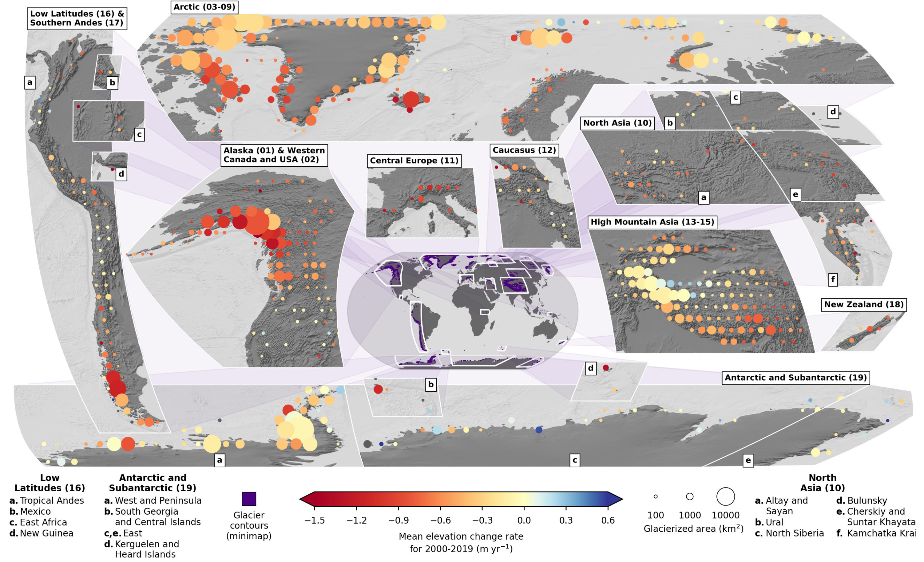

Number of valid observations per 100 m pixel per 5-year period on 1x1° tiles

./dataset/example_figs/alike_fig_ed7_datacov.py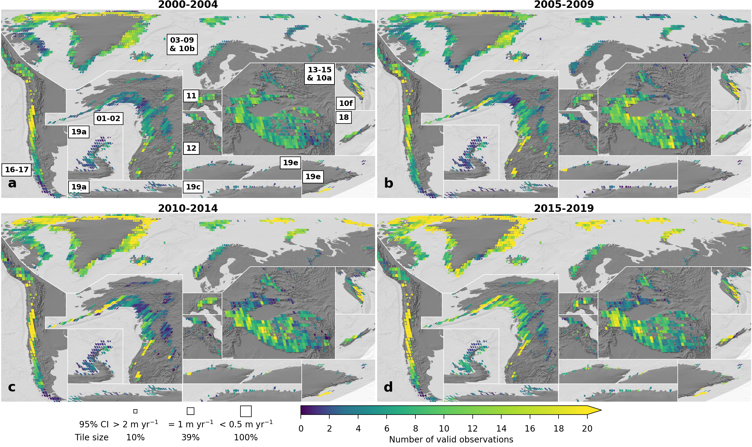

Mean elevation change rate per 5-year period on 0.5x0.5° tiles

./dataset/example_figs/alike_fig_ed7_05by05.py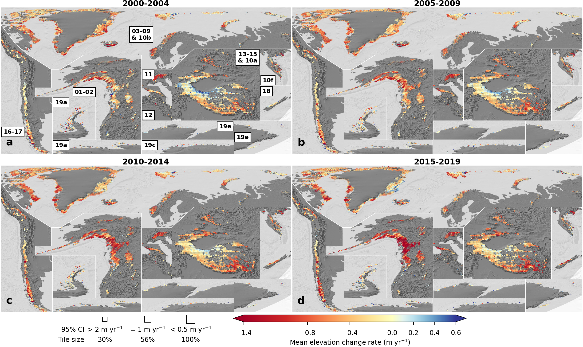

Mean elevation change rate per 2-year period on 1x1° tiles as a GIF

./dataset/example_figs/alike_fig_ed7_biennial_gif.py

As further guide, you will find comments directly present in the structure of the code, or in the documentation of our packages (pyddem, pymmaster).

Enjoy ! ⛄