In a 2008 crash analysis report, the state of Georgia had an estimate of 342,534 traffic accidents. Out of which, 133,555 individuals were injured, and 1,703 were dead. On average, Georgia faces around 1,000 traffic accidents per day.
One explanation for higher crash rates on Georgia roads is that extreme road conditions due to weather (e.g. rain, snow, ice) create potential safety hazards. Such potential safety hazards include, but are not limited to: driver(s) losing complete control of vehicle(s), improper lane changes, or obstruction of visibility. The United States Department of Transportation Road Weather Management Program reports that annual averages from 2007-2016 show 15% of vehicle crashes occurred due to wet pavements, 10% due to rain, 4% due to snow, and 3% due to ice [1].
Eliminating weather conditions and associated factors is not possible, however, understanding relations between conditions and crash risks could make drivers more aware of dangerous conditions. The following document presents an analysis of US traffic accidents surveyed over the span of several years with the intention of developing a severity assessment model, ie. How do weather conditions impact vehicle crash damage?
The dataset used for this project was found on Kaggle and put together by [2]-[4]. It contains 3.0 million records of spatial-temporal traffic accidents across 49 US states from February 2016 to December 2019. Among these records, variables such as time of day, latitute/longitude, weather conditions, road features were collected. This section summarizes the dataset's features and provides additional insight to its organization.
Shown below are the 49 original features each identified by their keyword as saved in the corresponding Pandas DataFrame:
| 1 | 2 | 3 | 4 | 5 | 6 | 7 | 8 | 9 | 10 |
|---|---|---|---|---|---|---|---|---|---|
| ID | Source | TMC | Severity | Start_Time | End_Time | Start_Lat | Stop_Lng | End_Lat | End_Lng |
| 11 | 12 | 13 | 14 | 15 | 16 | 17 | 18 | 19 | 20 |
| Distance(mi) | Description | Number | Street | Side | City | County | State | Zipcode | Country |
| 21 | 22 | 23 | 24 | 25 | 26 | 27 | 28 | 29 | 30 |
| Timezone | Airport_Code | Weather_Timestamp | Temperature(F) | Wind_Chill(F) | Humidity(%) | Pressure(in) | Visibility(mi) | Wind_Direction | Wind_Speed(mph) |
| 31 | 32 | 33 | 34 | 35 | 36 | 37 | 38 | 39 | 40 |
| Precipitation(in) | Weather_Condition | Amenity | Bumpy | Crossing | Give_Way | Junction | No_Exit | Railway | Roundabout |
| 41 | 42 | 43 | 44 | 45 | 46 | 47 | 48 | 49 | |
| Station | Stop | Traffic_Calming | Traffic_Signal | Turning_Loop | Sunrise_Sunset | Civil_Twilight | Nautical_Twilight | Astronomical_Twilight |
Several of the features have incomplete values or categorical values and will need to be cleaned up during preprocessing.
First we consider the distribution of samples across the entire dataset noting the following color map to indicate the four levels of crash severity that will be used as our supervised labels:

corresponding to a Severity of 1, 2, 3, and 4.
-
This map indicated the distribution of severity samples across the continental US.

-
The below histogram shows the crash occurance among each severity category. The imbalance in frequency among all four levels of severity will play an important role in our analysis.

- Additionally, the total quantity of accidents for each state is recorded.

-
This map indicated the distribution of severity samples across the state of Georgia.

-
The below histogram shows the crash occurance among each severity category.

As more and more Georgia drivers become aware of road conditions along their respective routes, there could be a significant reduction in the number of automotive accidents, injuries, and fatalities. Several predictive models are used to assess severity on Georgia roads that can be used to evaluate driving conditions in order to take necessary precautions.
In the study “A Perspective Analysis of Traffic Accidents using Data Mining Techniques” by S. Krishnaveni and Dr. Hemalatha, the researchers explored Naive Bayesian classifier, AdaBoostM1 Meta classifier, Random Forest Tree classifier, and PART Rule classifier to predict injury severity caused by traffic accidents in Hong Kong [5]. The research collected data based on accident (severity, weather, type of collision, road classification), vehicle (driver age, gender, manufacture date), and casualty (location of crash, degree of injury). As a result of this study, the Random Forest predictive model outperformed the other three models.
In our study, we have used relevant features such as weather conditions, time of day, and road layout to assess severity along Georgia roads. We first used Principle Component Analysis for dimensionality reduction then implemented Logistic Regression, Support Vector Machine, and Decision Tree classification models to see which model can best represent the datasets.
By implementing predictive machine learning models fed with informative data, Georgia users (drivers) can explore the most dangerous locations along their commutes during extreme weather conditions to either avoid or take extra precautions. Our study can also be extended to locations beyond Georgia, but for computational limitations, we focused on one state to explore.
During preprocessing, the data set is first cleaned up. This means:
- normalizing the data with respect to every feature
- filling in missing categorical data with the mode of that feature
- filling in missing numerical data with the median of that feature
- parsing date time objects by splitting them into year, month, day, hour, minute, and second attributes
- ex. 2016-02-08 06:07:59. Turns into month = 02, day = 08, weekday = 0 (Monday), hour = 06, minute = 07, second = 59.
- replacing True/False with 1/0
- applying one-hot encoding on categorical data
- ex. Sunrise_Sunset = {Day, Night}. Turn into Sunrise_Sunset_Day = {True, False}, Sunrise_Sunset_Night = {True, False}.
-
PCA aims to select principal components in a Z space in order to attain the largest possible variance.
-
Reduces dimensionality of data thereby reducing complexity.
-
For the original data set, each feature has some correlation/dependency on other features.

-
Applying PCA with 97% recovered variance resulted in the top 49 principal components.

-
The original correlation is removed after performing PCA. This is confirmed by the diagonal line in the resulting correlation analysis indicating the selected principal components are orthogonal to one another and thereby linearly independent (ie. not correlated).

Logistic regression in its basic form uses a logistic function to model a binary dependent variable. However, this algorithm can also be extended to model several classes of events.
Hyperparameters
-
Penalty: Specifies the type of normalization used. The default value l2 was used.
-
Inverse of regularization(C): Smaller values of this hyper-parameter indicates a stronger regularization. 1.0 was chosen based on literature and numerous trials.
-
Random state: Seed used by the random number generator. Default value of None was used.
-
Solver: Indicates which algorithm to use in the optimization problem. Default value of lbfgs was used.
-
Max iter: max_iter represents maximum number of iterations taken for the solvers to converge a training process. A value of 1000 was chosen.
Accuracy score = 0.527
For a multi-class problem such as this one, the sigmoid function is replaced by the softmax function. The softmax function tends to exaggerate small differences, potentially making the classifier biased towards a particular class even when it is not desired. Moreover, logistic regression does not perform well with variables that are very similar or correlated to each other. The presence of certain attributes that are similar and correlated to each other could've also caused this algorithm to not perform as well.
SVM maps data into a high dimension space so that decision boundaries can distinguish between the different classes.
Hyperparameters
- C (regularization)
- 100
(kernel coefficient)
- 1
Parameters
- kernel (kernel type)
- 'rbf' (radial basis function)
from sklearn.svm import SVC

svm = SVC(kernel='rbf', C=c, gamma=g).fit(X_train, y_train)

score_train = svm.score(X_train, y_train)
score_test = svm.score(X_test, y_test)

SVM struggled to fit onto the test after performing well on the training set, with 0.479 and 0.9997 accuracy, respectively.
An issue that was further researched is that SVM tends to work best for datasets consisting of fewer than 10,000 samples. Both training and testing sets were greater and therefore may have caused intense overfitting due to an inappropriate selection of the number of support vectors.
Gradient boosting combines small decision trees (relatively weak estimators) through a gradient descent algorithm rather than creating a single decision tree in order to produce a classification strong model that is robust to overfitting. Sk-learn has been implementing an experimental approach to gradient boosting using histograms to bin data and speed up calculations. This is the implementation we used.
Hyperparameters
- learning_rate
- max_iter
- max_leaf_nodes
- min_samples_leaf
- max_depth
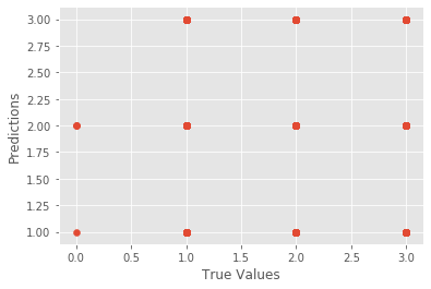
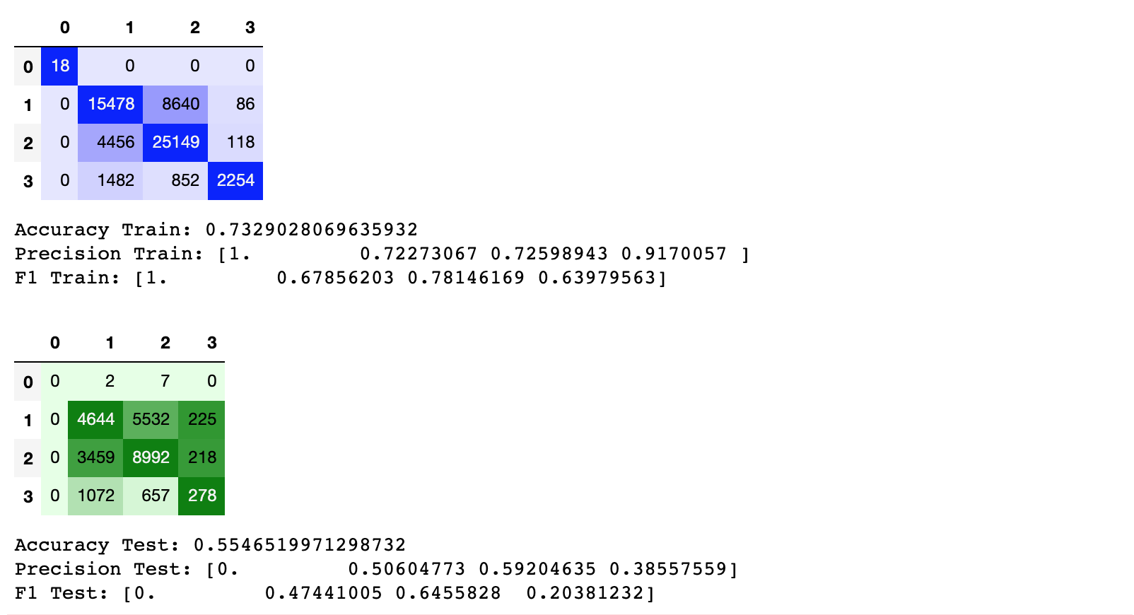
Results were first obtained with single iterations and some manual tuning of parameters. Further hyperparameter tuning was performed implementing sklearn.model_selection.GridSearchCV. Results shown (for comparing both training and test sets to their respective ground truths):
- Confusion Matrices
- Accuracy Score
- Prediction Score (for each individual label)
- F1 Score (for each individual label)
Hyperparameters for results shown:
- learning_rate: 0.1
- max_iter: 100
- max_leaf_nodes: default=20
- min_samples_leaf: 50
- max_depth: 8
Results:
Search Space explored:
- learning_rate: [0.05, 0.1, 0.15, 0.2]
- max_iter: [100, 500, 1000]
- max_leaf_nodes: default=20
- min_samples_leaf: [30, 50, 100]
- max_depth: [5, 6, 7, 8]
Due to time constaints, max leaf nodes was kept at default setting.
Results:
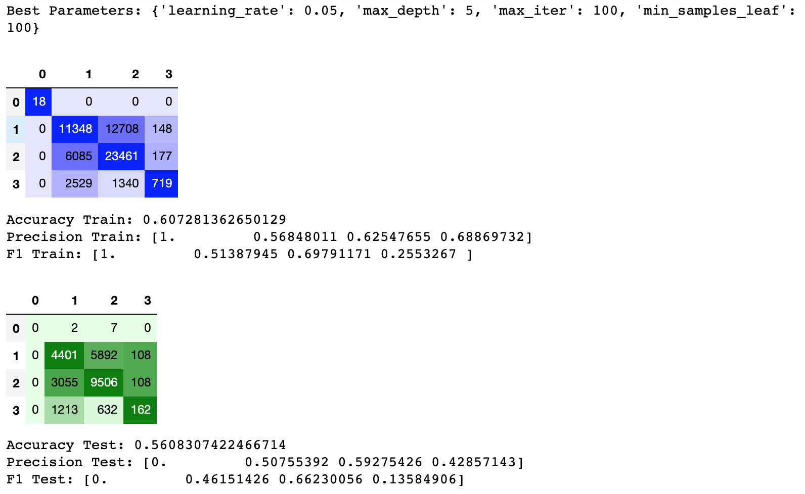
Gradient boosting is designed as a powerful combination of weak estimators that creates a model not as susceptible to overfitting as a standard decision tree. In this case, we can observe this through the relatively comparable accuracy, precision and F1 scores for training and test data. However, these scores remain fairly low. While some of these metrics tend to be harsh when looking at multilabel classification, the underlying bias of the traffic dataset towards severity 1 and 2 crashes (as well as an almost negligible amount of severity 0 scores) is a likely cause of the relatively low scoring metrics.
Further steps to improve the algorithm would include more directed hyperparameter tuning with a larger search space, as well as looking for ways to mitigate the skew of data (perhaps through stratified random sampling when constructing the training set to get more even numbers for each sample), and perhaps removing severity 0 traffic accidents entirely.
Overall, the project found some promise in its approach, but it is clear that a deeper investigation of the reported features is necessary. Another factor, mentioned during the dataset discussion, was that there was an imbalance in severity class with a heavy skew towards severity scores of 2 and 3. Future work and interest may consider grouping these classes into low and high opposed to the set {1, 2, 3, 4}. This requires a better understanding of how an accident was initially categorized during data collection. Future work lies in the interest to determine if local spatial classifiers are a better representation of vehicle accidents then the global spatial classifiers demonstrated. Since each physical location described by latitude and longitude features may be greater or less suspectible to weather conditions, a classifier across an entire state or even city may eliminate any distinctions.
-
[1] How do weather events impact roads? (2018). Federal Highway Administration. Retrieved from https://ops.fhwa.dot.gov/weather/q1roadimpact.htm
-
[3] Moosavi, Sobhan, Mohammad Hossein Samavatian, Srinivasan Parthasarathy, and Rajiv Ramnath. “A Countrywide Traffic Accident Dataset.”, arXiv preprint arXiv:1906.05409 (2019).
-
[4] Moosavi, Sobhan, Mohammad Hossein Samavatian, Srinivasan Parthasarathy, Radu Teodorescu, and Rajiv Ramnath. “Accident Risk Prediction based on Heterogeneous Sparse Data: New Dataset and Insights.” In proceedings of the 27th ACM SIGSPATIAL International Conference on Advances in Geographic Information Systems, ACM, 2019.
-
[5] Krishnaveni, S., & Hemalatha, M. (2011). A Perspective Analysis of Traffic Accident using Data Mining Techniques. International Journal of Computer Applications, 23(7), 40–48. doi: 10.5120/2896-3788