- In this repo we will cover all codes and revision needed for quick brush up for concepts.
- so that when we need to visit the concepts,its available for us.
The Structure is like
-
Data Types
-
Conditional statements 2.1 If loop 2.2 for loop 2.3 while loop
-
Functions and variables
-
Classes
-
Reading files
-
Strings
-
functions and files
-
memorizing logic
1.Data Types
There are seven data types in python. Let's have a look at them with direct examaple for better understanding.
boolean = True
number = 1.1
string = "Strings can be declared with single or double quotes."
2. Conditional statements
2.1 If else Loop:
   ```
   password = raw_input("Enter the password")
   if password =="MI6":
      print("welcome Mr.bond")
   else:
      print("access denied")
   ```
Let's check what is if...else loop.
if condition-1:
      sequence of statements-1
elif condition-n:
      sequence of statements-n
else:
      default sequence of statements
The conditionals can also be represented by following code snippet.
if cake == "delicious":
   return "Yes please"
elif cake == "Okay":
   return "I will have a small piece"
else:
   return "No,Thank You"
Now, let's try to put college grades into use and understand how we can put the grades through programming:
| Grdaes | Score |
|---|---|
| A | All grades above 4 |
| B | All grades above 3 and below 3.5 |
| C | All grades above 2.5 and below3 |
| D | All Grades below 2.5 |
 num = float(input("Enter the number:"))

 if num > 4:
     letter = "A"
 elif num > 3:
    letter = "B"
 elif num > 2:
    letter = "C"
 else:
    letter = "D"
 print("The grade is",letter)
2.2 For Loop:
The simple example of for loop can be given as:
for item in list:
   print item
It prints all the items in list
suppose, list=[1,2,3,4,5,6], "item" is new variable created at runtime. Then it is referenced to array(list) index and printed using {print item} line.
The output is=> [1,2,3,4,5,6]
2.3 While Loop:
While loop is run until the condition is true. When it becomes FALSE the loop terminates.
for example:
while (total < max_val):
   total += values[i]
   i+=2  # i is incremented by two. Due to this condition becomes false & loop terminates.
3. Functions
Let's try to understand functions in new way.
def divide(dividend, divisor):
      quotient = dividend/divisor
      remainder = divident % divisor
      return quotient, remainder
This is the generalised code for division. Here,the primary goal is to understand how functions work. Functions are nothing but blocks of code which when called run the block with provided parameters and returns data as a result.
How to call function: Function can be called using their name and parenthesis. For example:
divide(25,5)
# here it takes two params hence we passed 25 and 5

divide(45,5)
# here also it takes 2 parameters
4. Classes:
Class is something that it's like a home to functions and objects. Class bundles data and functionality together.
For Ex:
   def __init__(self,name,age):
      self.name = name
      self.age = age

   def birthday(self):
self.age +=1 -
List based collections
1.1 Lists/Arrays
1.2 Linked Lists
1.3 Stacks
1.4 Queues -
Searching and Sorting
2.1 Binary Search
2.2 Recursion
2.3 Bubble Sort
2.4 Merge Sort
2.5 Quick Sort -
Maps and Hashing
-
Trees
-
Graphs
-
Case Studies in Algorithms
-
Technical Interview Tips
1.1 Lists:
Python has an interesting data stucture called a "list" that is much more than a mere list. Behind the scenes a Python list is built as an array. Even though you can do many operations on a Python list with just one line of code, there's a lot of code built in to the Python language running to make that operation possible.
For example, inserting into a list is easy (happens in constant time). However, inserting into an array is O(n), since you may need to shift elements to make space for the one you're inserting, or even copy everything to a new array if you run out of space. Thus, inserting into a Python list is actually O(n), while operations that search for an element at a particular spot are O(1).
Python is a "higher level" programming language, so you can accomplish a task with little code. However, there's a lot of code built into the infrastructure in this way that causes your code to actually run much more slowly than you'd think. Keep this in the back of your mind when using Python.
You likely won't need to know the details of how Python works behind the scenes in a programming interview, but you'll seem very impressive if you do!
1.2 Linked Lists:
- Linked List is extension of list but it's definitely not an array. A Linked List is characterised by it's links.
- Each elements has some notion of what the next element is since it's connected to it, but not necessarily how long the list is or where it is in the list.
- Linked list has a memory location of next block for traversing purpose and that block has memory location of next block and so on.
- The blocks in linked list should be connected and if any link is missing then traversing becomes difficult.
Single unit linked list examaple
class Element(object):
  def __init__(self, value):
     self.value = value
     self.next = None
Before moving on lets understand it. We use __init__ to initialize a new Element. An Element has some value associated with it (which could be anything—a number, a string, a character, et cetera), and it has a variable that points to the next element in the linked list.
Let's see how to setup LinkedList class
class LinkedList(object):
      def __init__(self,head=None):
self.head = head- This code is very similar— we're just establishing that a LinkedList is something that has a head Element, which is the first element in the list. If we establish a new LinkedList without a head, it will default to None.
Let's build one method to append new elements at end of LinkedList
class append(self,new_element):
      current = self.head

      if self.head:
         while current.next:
            current = current.next
         current.next = new_element
      else:
self.head = new_element-
If LinkedList already has a
head, we iterate through thenextreference in everyElementuntil we reach the end of the list. -
Set
nextfor the end of the list to thenew_element. Alternatively, if there is no head already, you should just assign new_element to it and do nothing else.
1.3 Stacks:
Stack is a data structure in python which is based on LIFO( Last In First Out).
It has two methods
- push()
- pop()
push() is used when we need to add element in stack.
Similarly, when we need to remove an element from stack we use pop() method.
1.4 Queues:
Unlike stack queue is a linear data structure that stores elements is FIFO order i.e First In First Out. The recently added item in Queue is removed last. A quick example to visualize is queue of person at ticket box. The person who comes first is served first and the last one is served last.
Operations in Queue:
- Enqueue:
In this operation we add elements to queue. If the queue is full then it's called as overflow.
- Dequeue:
The operation of removing elements from queue is called Dequeue. The items are removed in same fashion as they have entered in queue.
Priority Queue : Priority queue is also type of queue in which less popular elements are placed in front and more popular elements are place at the back.
-
In order to implement algorithms in programming languages, you will need to understand an algorithm in detailed.
-
Human may know how algorithm works but we need the computers to know how algorithms work as computers are going to execute it.
2.1 Binary Search:
-
Binary search is the efficient algorithm for finding an item from sorted or unsorted array. The most common ways to use binary search is to find an item in array.
-
Basically an algorithm is just high level description of a trick of solving a problem.
-
If all the names in the world are written down together in order and you want to search for the position of a specific name, binary search will accomplish this in a maximum of 35 iterations.
-
It works on only sorted set of elements.
-
while performing opearion on binary search, the total number of iterations may vary depending upon the number to be searched.
-
Let's consider following array:
-
By using linear search, the position of element 8 will be determined in the 9th iteration.
-
Let's see how to reduce the number of iterations using binary search. For that we need to knoe the start and end of the range. Let's call them
LowandHigh
Low  = 0
High = n-1-
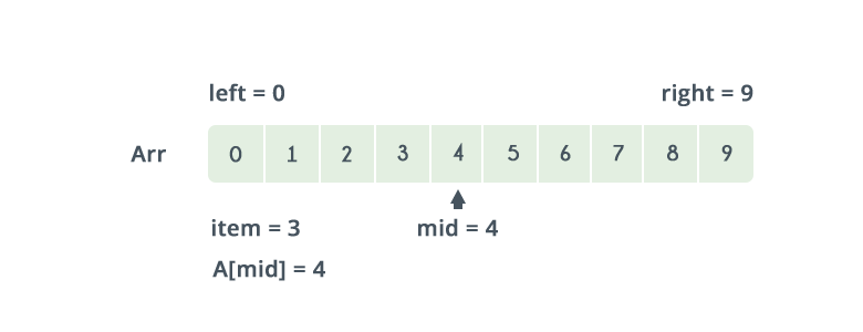
Now we compare the Search value K with the element located at the center of lower bound and upper bound.
-
If value of K is greater then increase the lower bound else decrease the lower bound.
-
As per above image, Lower bound = 0. The median is calculated as (lower bound + upper bound) \2 =4.
-
Value of a[4]=4. The value 4>2, and this is the element you are searching for.
-
Hence, no need to conduct search on any element beyond 4 as the elements beyond it will obviously be greater than 2.
-
Therefore, we can drop the upper bound of the array to position of element 4. Now we follow the same procedure on the same array with following values.
Low:  0
High: 3-
Repeat the procedure until Low > High.
-
If at any iteration we get a[mid] = key, we return value of mid. This is the position of key in array. If key is not present in array, we return -1.
-
Let's have a look at implementation.
int binarySearch(int low,int high, int key):
{
   while(low <= high)
   {
      int mid = (low+high)/2;

      if(a[mid]<key)
      {
         low=mid+1;
      }
      else if(a[mid]>key)
      {
         high = mid-1;
      }
      else
      {
         return mid;
      }
   }
   return -1;  //key not found
}
Time complexity: Worst case time complexity is O(log2N).
Python Program for recursive binary Search:
-
Compare x with the middle element.
-
If x matches with the middle element, we return the mid index.
-
Else if x is greater than the mid element, then x can only lie in the right (greater) half subarray after the mid element. Then we apply the algorithm again for the right half.
-
Else if x is smaller, the target x must lie in the left (lower) half. So we apply the algorithm for the left half.
def binary_search(arr,low,high,x):

   if high >= low: #base case

      #calculate mid
      mid =(low+high)//2

      #If element is present at the middle
      if arr[mid]==x:
         return mid
      #if element is smalleer than mid then it can only be present at the left side
      if arr[mid] > x:
         return binary_search(arr,low,mid-1,x)

      #else element is in the right sub-array

      else:
         return binary_search(arr,mid+1,high,x)

   else:
      return -1 #element is not present in the array.

#test array
arr=[2,3,4,10,40]

x=10

#make function call
result= binary_search(arr,0,len(arr)-1,x)

if result != -1:
   print("Element is present at index", str(result))
else:
   print("Element is not present in array")


# output: Element is present at index 3
2.2 Recursion:
-
Recursion is process of defining something in terms of itself.
-
In real world for ex we can take two mirrors facing each other.Any object between them would be reflected recursively.
python recursive function:
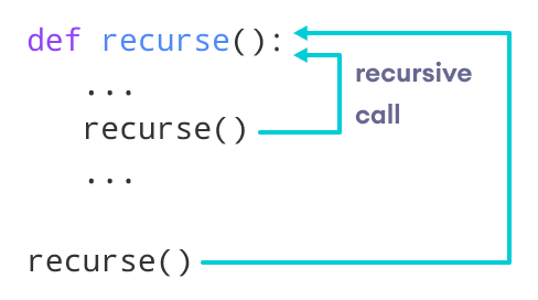
In python, we see that a function can call another function. Likewise it's also possible for function to call itself. This concept is known as Recursive functions
The following image shows working of recursive function.
- Let's see the example of factorial which is a recursive function.
Example:
def factorial(x):

   if x ==1:
      return 1
   else:
      return (x*factorial(x-1))

num=4
print("Factorial of ",num,"is",factorial(num))
Output: Factorial of 4 is 24
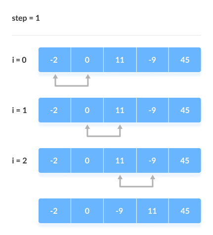
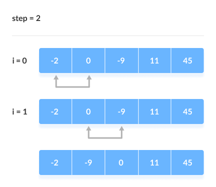
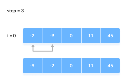
2.3 Bubble Sort:
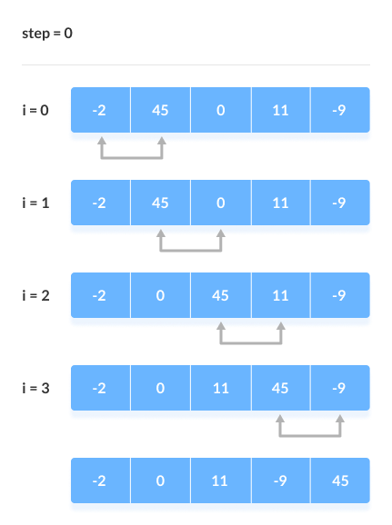
Bubble sort is also known as comparison sort,is a simple sorting algorithm. It repetitively goes throught the list and swaps the adjacent elements which are in the wrong order.
How bubble sort works:
- Starting from the first index, compare the first and the second elements.If the first element is greater than the second element, they are swapped.
- Now, compare the second and the third elements. Swap them if they are not in order.
- This process continues till the last element.
For ex: See the given Image
- The same process goes on for the remaining iterations.
- After each iteration, the largest element among the unsorted elements is placed at the end.
- In each iteration, the comparison takes place up to the last unsorted element.
- The array is sorted when all the unsorted elements are placed at their correct position.
Bubble Sort Algorithm:
bubbleSort(array)
   for i <- 1 to indexOfLastUnsortedElement -1
      if leftElement > rightElement
         swap leftElement and rightElement
end bubbleSort
Python Implementation:
def bubbleSort(array):
    for i in range(len(array)):
        for j in range(0,len(array)-i-1):
            #sort
            if array[j] > array[j+1]"
                #swap if greater elem is at rear position
                (array[j],array[j+1]) = (array[j+1],array[j])


data = [5,0,14,1,25]
bubbleSort(data)
print("sorted arraty is ascending order:")
print(data)
2.4 Merge Sort:
-
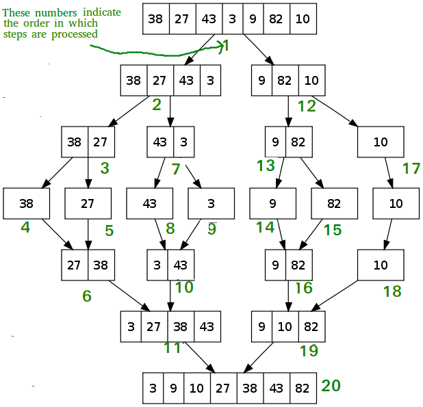
Merge Sort is based on Divide and Conquer strategy. It divides the input array into two halves, calls itself for the two halves, and then merges the two sorted halves.
-
The following diagram from wikipedia shows the complete merge sort process for an example array {38, 27, 43, 3, 9, 82, 10}.
-
If we take a closer look at the diagram, we can see that the array is recursively divided in two halves till the size becomes 1.
-
Once the size becomes 1, the merge processes come into action and start merging arrays back till the complete array is merged.
we are following the below approach:
MergeSort(arr[],l,r)

If r > l
      1. Find the middle point to divide array into two parts:
               middle = (l+r)/2
      2. call MergeSort for firsh half:
               call MergeSort(arr,l,m)
      3. call MergeSort for second half:
               call MergeSort(arr,m+1,r)
      4. Merge the two sorted halves in step 2 & 3:
               Call merge(arr,l,m,r)
Code Implementation:
def mergeSort(arr):
   if len(arr) >1:

      #find the middle of tha array
      mid = len(arr)//2

      #divide the array elements
      L = arr[:mid]

      #into 2 parts
      R= arr[mid:]

      #sorting first half
      mergeSort(L)

      #sorting second half
      mergeSort(R)

      i = j = k = 0

      #copy data from temp arrays L[] and R[]

      while i< len(L) and j < len(R):
         if L[i] < R[j]
            arr[k]=L[i]  # putting value of first element of array L into array K
            i+=1
         else:
            arr[k] = R[j] # else put array R's first element in array K.. simple
            j +=1
         k=k+1

      #checking if any element was left
      while i< len(L):
         arr[k] = L[i]
         i+=1
         k+=1

      while j< len(R):
         arr[k] = R[j]
         j+=1
         k+=1

# code to print  the list

def printList(arr):
   for i in range(len(arr)):
      print(arr[i],end="")
   print()

#main diver code

if __name__== '__main__':
   arr = [12,11,13,5,6,7]
   print("given array is",end="\n")
   printList(arr)

   mergeSort(arr)
   print("Sorted array is:", end="\n")
   printList(arr)
Time Complexity:
Merge sort is recursive algorithm and time complexity can be expressed as T(n) = 2T(n/2)+θ(n)
- The above recurrence can be solved either by using the Recurrence Tree method or the Master method. It falls in case II of Master Method and the solution of the recurrence is
θ(nLogn). - Time complexity of Merge Sort is
θ(nLogn)in all 3 cases (worst, average and best) as merge sort always divides the array into two halves and takes linear time to merge two halves.
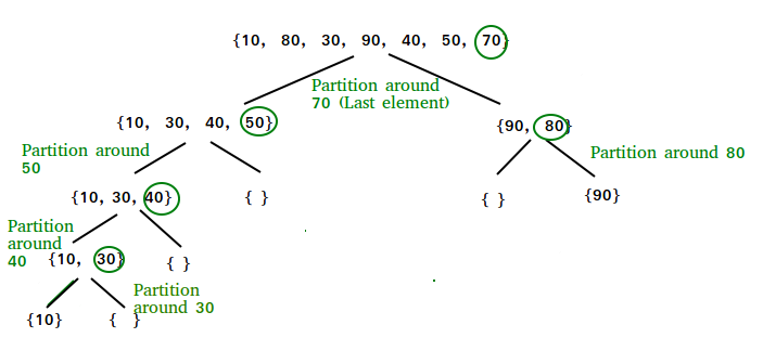
2.5 Quick Sort:
-
The quick sort uses divide and conquer to gain the same advantages as the merge sort, while not using additional storage. As a trade-off, however, it is possible that the list may not be divided in half. When this happens, we will see that performance is diminished.
-
A quick sort first selects a value,which is pivot value. There are many ways to choose pivot value but we simply use the first value. The role of pivot value is to assist with splitting list.
-
The actual position where the pivot value belongs in the final sorted list, commonly called the split point, will be used to divide the list for subsequent calls to the quick sort.
-
Different versions of quickSort that pick pivot in different ways.
- Always pick first element as pivot
- Always pick last element as pivot
- pick a random element as pivot
- pick median as pivot
PseudoCode for recursive Quicksort function:
#low -> start index
# high -> end index

quicksort(arr[],low,high):
   if low < high:
      # pi is partitioning index, arr[pi] is now at right place

      pi= partition(arr,low,high)

      quicksort(arr,low,pi-1)   # before pi
quicksort(arr,pi + 1,high)# after pi- Let's have a look at following figure:
- Below Video will help you to visualize the process:
quick sort reference: https://runestone.academy/runestone/books/published/pythonds/SortSearch/TheQuickSort.html
-
Hash maps are indexed data structures. A hash map makes use of a hash function to compute an index with a key into an array of buckets or slots. It's values is mapped to the bucket with corresponding index.
-
The key is unique and immutable(can not be changed). Think of hashmap as bottles with the labels of liquid item stored in them.
-
Hash function is the core of implementing Hash Map.
-
It takes the key and translates it in to the index of bucket in bucket list.
-
Ideal hashing should produce a different index for each key. However, collisions can occur. When hashing gives same/existing index, we can simply use a bucket for multiple values by appending the list or byb rehashing.
-
In python, dictionaries can be considered as examples of hash maps.
-
The Hashmap design will include following functions:
set_val(key,value): get_val(key): delete_val(key):
Let's have a Look at Implementation:
class HashTable:

    def __init__(self,size):
      self.size=size
      self.hashtable = self.create_buckets()


    def create_buckets(self):
      return [[] for _ in range(self.size)]

    #insert value into hashmap

    def set_val(self,key,value):
      # now get the index from key using hash function

      hashed_key= hash(key) % self.size

      #get the bucket correspoding to index.
      bucket = self.hash_table[hashed_key]

      found_key = False

      for index,record in enumerate(bucket):
        record_key,record_val = record

        #check if the name has the same key to be inserted.
        if record_key == key:
          found_key = True
          break

      '''
      if the bucket has same as the key to be inserted,
      update the key value
      otherwise append the new key-value pair to the bucket
      '''
      if found_key:
         bucket[index] = (key,val)
      else:
         bucket.append((key,val))

    #return searched value with specific key
    def get_val(self,key):

      #Get the index from the key using hash function
      hashed_key = hash(key) % self.size

      #Get the bucket corresponding to index
      bucket = self.hash_table[hashed_key]

      found_key = False

      for index,record in enumerate(bucket):
         record_key, record_val = record

         # check if the bucket has the same key as the key being searched

         if record_key == key
            found_key =True
            break

      #if the bucket has same key as the key being searched,
      #return the value found
      # Otherwise indicate there was no record found

      if found_key:
         return record_val
      else:
         return "No record Found"

    #remove a value with specific key

    def delete_val(self,key):
      #get the index from the key using hash function

      hashed_key= hash(key) % self.size

    #Remove a value wit specific key

    def delete_val(self,key):
      #get the index from the key using hash function

      hashed_key = hash(key) %self.size

      #get the bucket corresponding to index
      bucket = self.hash_table[hashed_key]

      found_key=False
      for index,record in enumerate(bucket):
        record_key, record_val= record

        #check if the bucket has the same key as to be deleted
        if record_key  == key:
          found_key = True
          break

      if found_key:
        bucket.pop(index)
       return

     # to print the items of hash map

     def __str__(self):
      return "".join(str(item) for item in self.hash_table )


hash_table = HashTable(50)

#insert values

hash_table.set_val("Rock","rock11@gmail.com)
print(hash_table)
print()

hash_table.set_val("Tom","tomcruize@gmail.com)
print(hash_table)
print()

hash_table.set_val("ben","ben.obama@gmail.com)
print(hash_table)
print()


#search / access the record using key

print(hash_table.get_val('Rock'))
print()

print(hash_table.get_val('Tom'))
print()

#delete or remove a value

hash_table.delete_val('Rock')
print(hash_table)
Time Complexity:
Memory index access takes constant time and hashing takes constant time. Hence, the search complexity of hash map is also constant time, i.e. O(1)
-
Trees are non-linear Data Structure.
-
we know linked list,similarly trees are made up of nodes. A common kind of tree is Binary Tree, in which each node contains a reference to two other nodes (posibly none). These reference are referred to as the left and right subtree.
-
The top node is called as root (main node), the other nodes are called branches and the nodes which are at tips with null reference are called leaves
-
Top nodes are sometimes also called as parent and the nodes below parent are referred as children Nodes.
-
Nodes with same parent are called siblings.
-
Nodes having different parents but same grand parents are called Cousins.
-
We already mentioned right and left, but there is up(towards root/parent) and down(leaves/childrens) also.
-
Trees are considered as recursive data structure reason being they are defined recursively. A tree is either
- the empty tree, represented by
NONEor - a node conatining an object reference and two tree references.
- the empty tree, represented by
-
In a tree having N nodes there will be exactly N-1 edges.

-
Depth of node x in tree is defined as lenght of the path from root to x. Each edge in the path will contribute for one unit in length.
-
Depth of root node is Zero.
-
Height of any node in tree is defined as number of edges in longest path from that node to a leaf.
- We build the tree through same process as we build linked list. Each constructor invocation builds a single node.
class tree:

  def __init__(self,cargo,left=None,right=None):
    self.cargo=cargo
    self.left= left
    self.right=right

  def __str__(self):
return str(self.cargo) -
the cargo can be of any type,but the left and right parameteres should be tree nodes.
leftandrightare optional,thedefafult value isNone. -
To print the cargo we have to just print the cargo.
-
There is one more way to build the tree, its bottom up way i.e. allocating the child nodes first.
left = Tree(2)
right= Tree(3)- Now we add Parent node and link it to the childrens
tree = Tree(1,left,right)- Another way is by nesting constructor invocations
tree = Tree(1,Tree(2),Tree(3))- We always want to traverse any data structure that comes across us. Same way the most simple way to traverse Tree is recursively.
- For Example, if the tree contains integers as cargo, the below function will return their sum.
def total(tree):
  if tree == None: return 0
return total(tree.left) + total(tree.right) +tree.cargo- Base case is empty tree, it contains no cargo,so the sum is zero.
- The recursive step makes two recirsive calls( one to left subtree & second to right subtree) to find the sum of child subtrees.
- When the recursive calls complete then we add the cargo of parent and return the total.
- Tree is natural way to represent the structure of an expression. Unlike other notations, it represents the computations unambiguously.
- For Example, the infix expression
1 + 2 * 3is ambiguous unless we know that the multiplication happens before addition. - The expression trees represent the same computation.
- The nodes of such expression trees are operands like 1,2,3 or operators like + and *. Operands are leaf nodes.
- Operator nodes have refr=erences to their operands. (All of these opearators are binary, meaning they have exactly two operands.
- We can build tree like this:
tree = Tree ('+', Tree(1), Tree(' * ' , Tree(2), Tree(3)))
- order of operation is- the multiplication is first and then second opearation of addition.
- These expression Trees can be used to convert expressions like postfix,prefix,infix to each other.
- we can traverse the expression trees and print the content like this:
def print_tree(tree):
   if tree == None: return
   print tree.cargo,

   print_tree(tree.left)
print_tree(tree.right)- To print the tree, we first print the root,then left subtree and then right subtree.
- This way of traversing the tree is called as Preorder as root is accessed or printed before the children.
- For the previous example the output is:
tree = Tree('+', Tree(1), Tree(' * ' , Tree(2), Tree(3)))
print_tree(tree)
Output
+ 1 *2 3
-
This expression is called as prefix, in which operator appears before operands.
-
If we traverse the tree in different order we will get the expression in different notation.
-
For Ex:
def print_tree_postorder(tree):
   if tree==None: return

   print_tree_postorder(tree.left)
   print_tree_postorder(tree.right)
print tree.cargo-
The result is
1 2 3 * +. This order of traversal is called as post order traversal. -
Now, to traverse the tree Inorder, print the left tree, then root and then right tree.
def print_tree_inorder(tree):
   if tree == None:return

   print_tree_inorder(tree.left)
   print tree.cargo
print_tree_inorder(tree.right)- The result is
1 + 2 * 3, which is the infix expression. - Inorder traversal is not that sufficient to generate an infix expression.
-
In this part, we parse infix expression and build the corresponding expression Trees. For example, the expression
(3 + 7) * 9yields one tree. -
The parser we are writing will handle the expression that includes numbers, parentheses, and the operators + and *. We assume that the input string has already been tokenized into a python list(producing the list is the task given to you).
-
the token list for (3+7) *9 is:
['(',3,'+',7,')', '*', 9, 'end']-
The end token is necessary to prevent the parser from reading further list
-
We are going to write one function for it.
-
The function is will take token_list and expected token as parameters. Then it will compare the expected token to the first token in the list.
-
If they match,it removes the token from list and returns
TrueelseFalse
def get_token(token_list,expected):
   if token_list[i] == expected:
      del token_list[i]
      return True
   else:
return False-
token_list refers to mutable object, the changes made here are visible to any other variable that refers to the same object.
-
The next function is
get_number. It handles the operands. -
If the next number in token_list is number then get_number() removes it and returns leaf node containing number,Otherwise it returns None.
def get_number(token_list):
    x =token_list[0]
    if type(x) != type(0):return None
    del token_list[0]
    return Tree (x, None,None)
- Before moving ahead we should test the get_number() function.
- we assign list of numbers to token_list.
token_list = [9,11,'end']
x= get_number(token_list)
print_tree_postorder(x)

print token_list
__OUTPUT:__
[11,'end']
-
The next method is get_product, which builds an expression tree for products. A simple product has two numbers as operands like 3 x 7
-
Let's see the code of get_product.
def get_product(token_list):
  a = get_number(token_list):
  if get_token(token_list, "*"):
    b= get_number(token_list)
    return Tree('*' , a,b)
  else:
return a- We assume that get_number succeeds and returns a singleton tree.
- We have assigned first operand to a. If the next character is * , we get the second number and are ready to build the expression tree with a,b and operator.
- If the next character is other than expected then we return the leaf node with a.
For Example:
1
> token_list = [9,'*',11,'end']
> tree = get_product(token_list)
> print_tree_postorder(tree)

9 11 *
2
> token_list = [9,'+',11,'end']
> tree = get_product(token_list)
> print_tree_postorder(tree)

9
-
In second Example, there is '+' operator than ' * ' so we returned only leaf(a=9)
-
Now we have to deal with compund products,like
3*5*13. We treat this expression as product of products, like3 * (5 * 13). -
By making a small change in
get_productwe can handle such long products. -
Let's see the code for that.
def get_product(token_list):
    a= get_number(token_list)
    if get_token(token_list,'*'):
        b=get_product(token_list)     # this line changed. recursive call
        return Tree('*', a ,b )
    else:
        return a
- In other words, a product can be eithera singleton or tree with * at the root, a number of the left, and a product on the right.
- Let's test a new example with compound product.
> token_list = [2, '*', 3, '*', 5, '*', 7, '*', 'end']

> tree = get_product(token_list)

> print_tree_postorder(tree)

output: 2 3 5 7 * * *-
Coming to next point we can add ability to parse the sums.
-
For us sum can be a tree with
+at root, a product on the left and sum on the right or a sum can be just a product. -
There is one interesting property called as basis of parsing algorithm.
-
With its help we can represent any expression without parenthesis as sum of products.
-
get_sum()function tries to build a tree with a product on the left and sum on the right. But if it doesn't find a +, it just builds a product. -
Let's have a look at example;
def get_sum(token_list):
   a = get_product(token_list)
   if get_token(token_list, '+'):

      b=get_sum(token_list)

      return Tree ('+', a, b)
   else:
return a- Now we have to test it with
9 * 11 +5 *7
> token_list = [9, '*', 11, '+', 5, '*', 7, 'end']
> tree = get_sum(token_list)
>print_tree_postorder(tree)

Output:


9 11 * 5 7 * +
- Finally, we will move towards handling parenthesis.
- Anywhere in the expresion Where there can be a number ,there can be an entire sum enclosed in parenthesis.
def get_number(token_list):
    if get_token(token_list, '(' ):
        x = get_sum(token_list)       # get the sub expression
        get_token(token_list,')')     # remove the closing parenthesis
        return x
    else:
        x = token_list[0]
        if type(x) != type(0): return None
        token_list[0:1] = []
        return Tree(x,None,None)
- So this is how we build expression trees in python.
Binary Tree Binary search tree AVL Tree